
Dr Ajay Kumar Koli
Head & Educator
School of Information & Data Science
Nalanda Academy - Wardha
@ajay_kolii
koliajaykumar@gmail.com
https://koliajay.netlify.app/
Hello! 😊
😍 R is FREE
R is a language and environment for statistical computing and graphics. (R project)
In August 1993, designed by

Ross Ihaka
(New Zealand Statistician)

Robert Gentleman
(Canadian Statistician)
Download R from CRAN

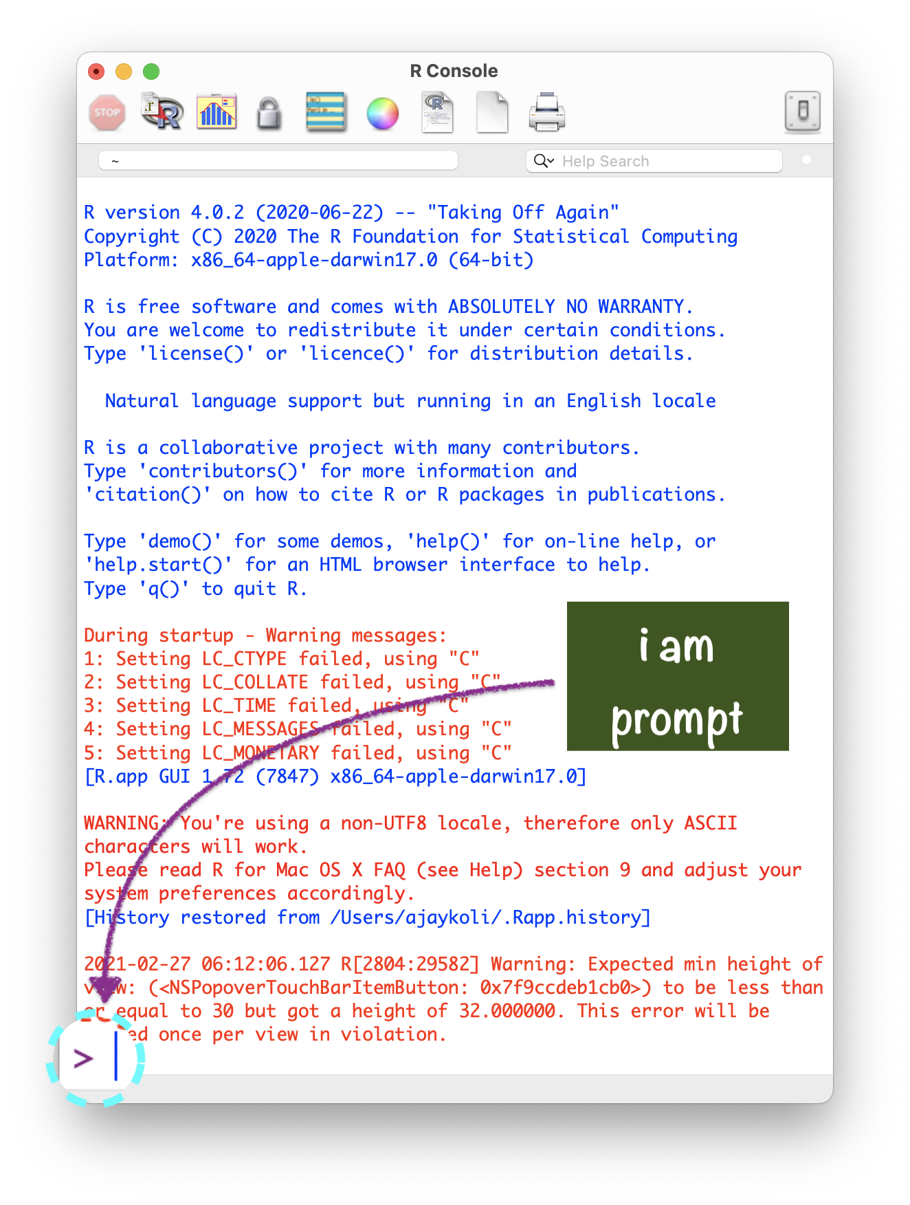
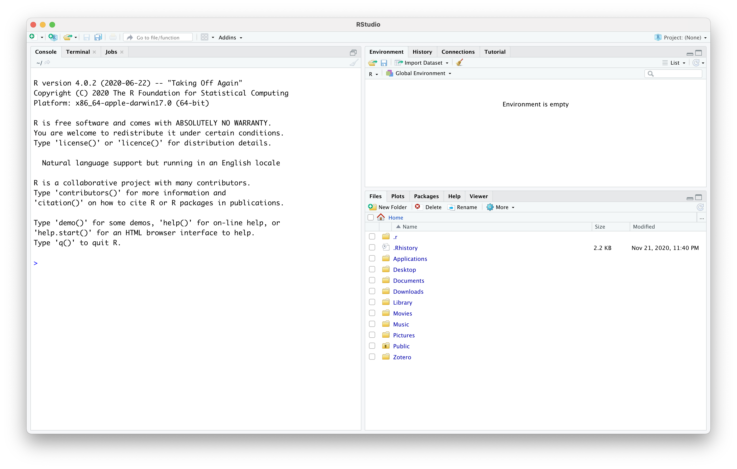
R Console
- R version
- R name
- R licence
- prompt >
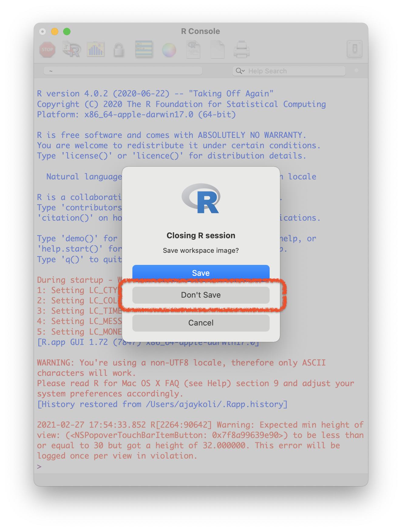
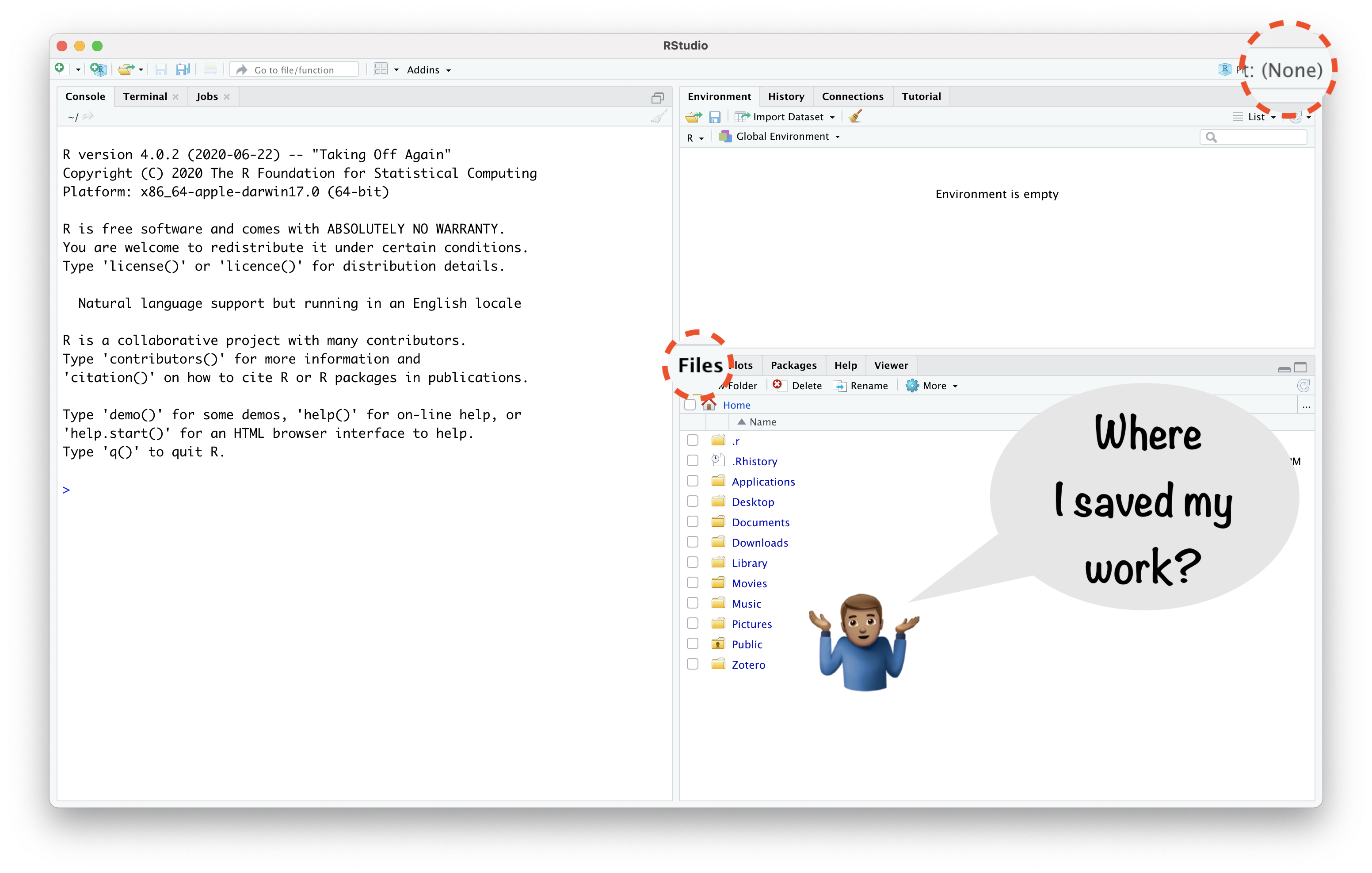
Never Save R "Workspace Image":
It helps in "freshly minted R sessions".
"put more trust in your script than in your memory"
RStudio IDE
RStudio \(\rightarrow\) Tools \(\rightarrow\) Global Options
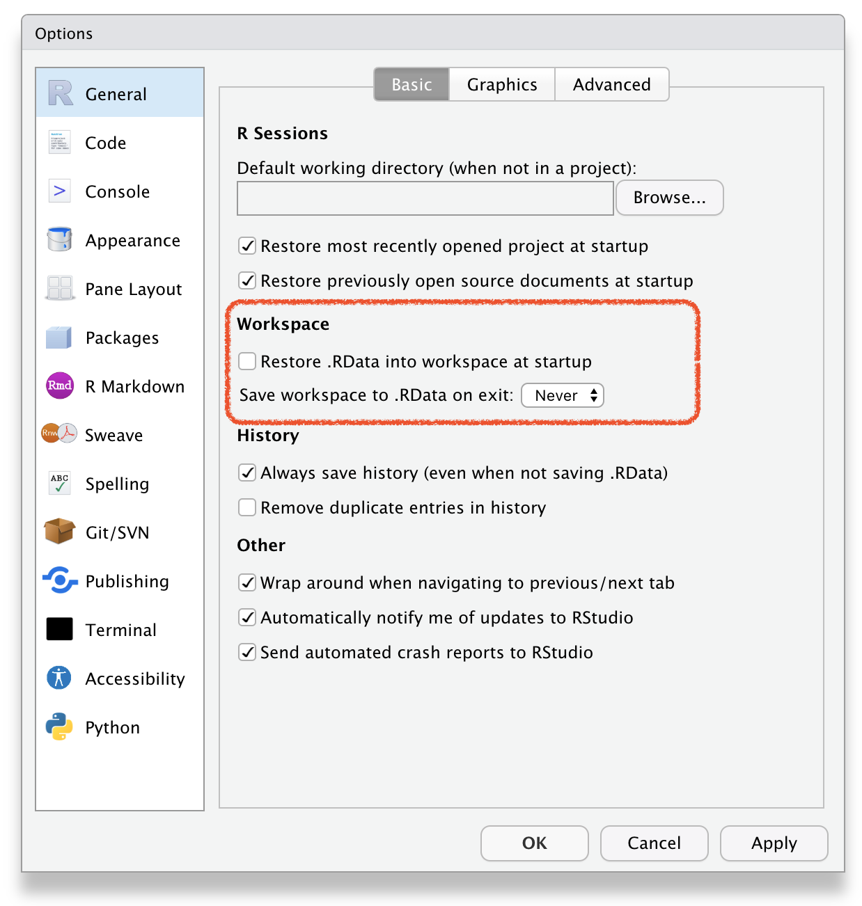
RStudio \(\rightarrow\) Tools \(\rightarrow\) Global Options
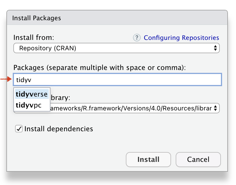
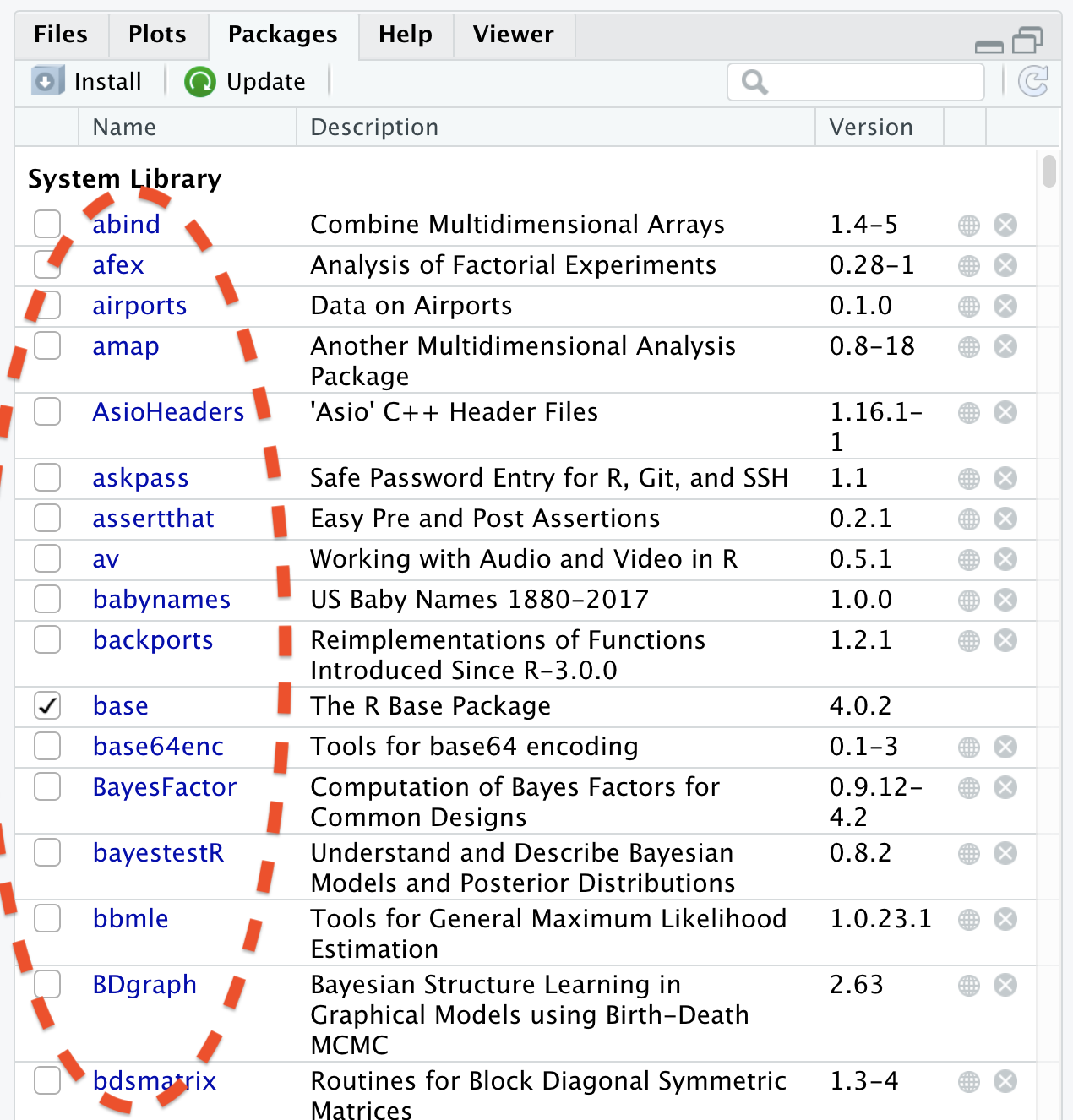
To Download pkgs
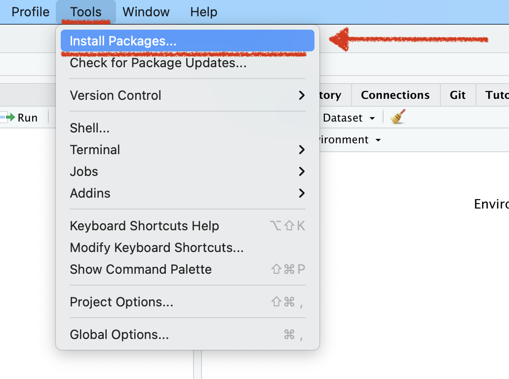
Name of the R package(s)
Installed R package(s)
Tools \(\rightarrow\) Check Package Updates
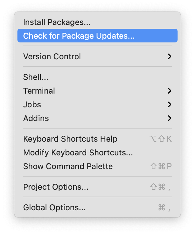
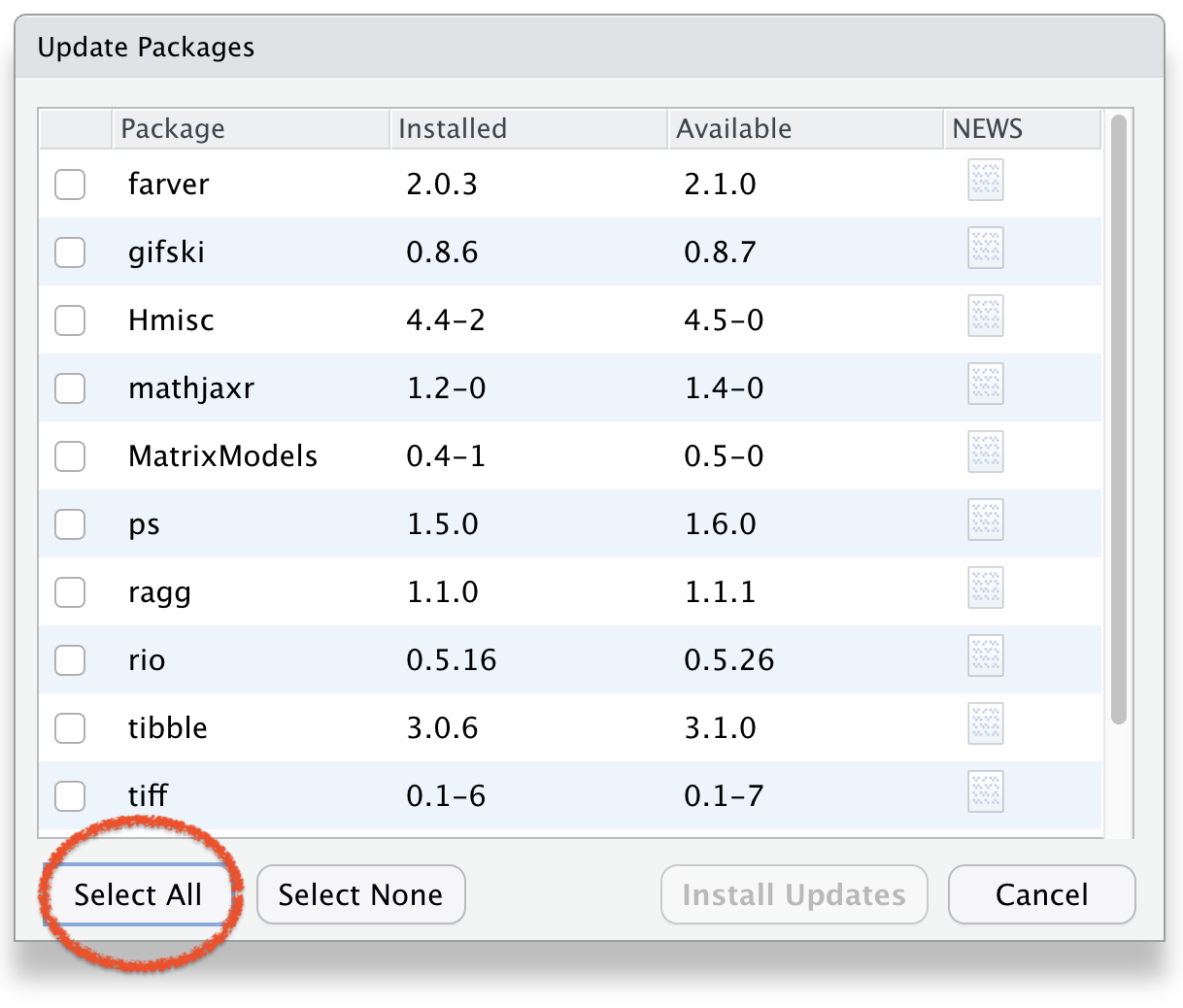
Select Package(s) to Update
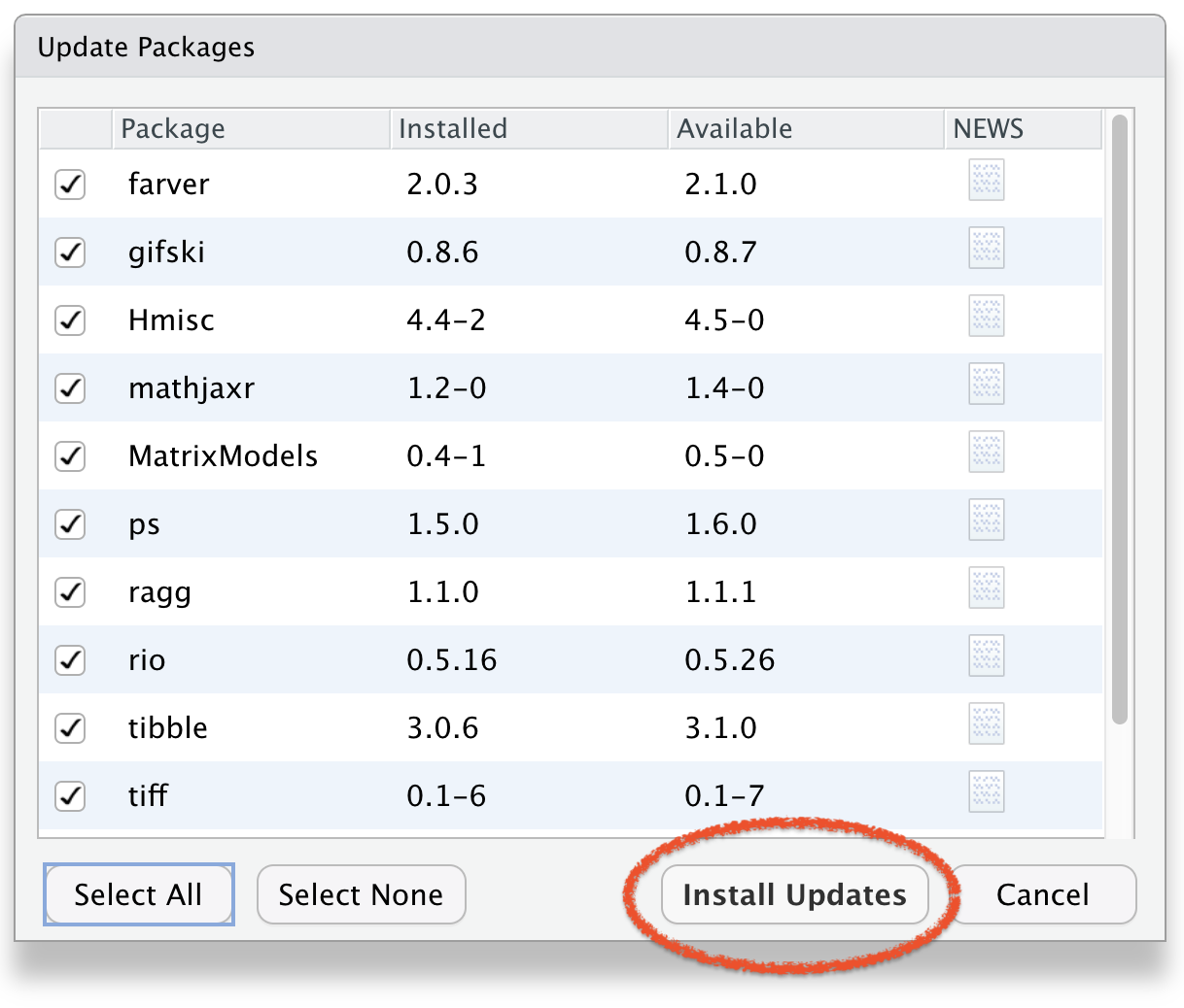
Click Install Updates
To Remove Package(s)
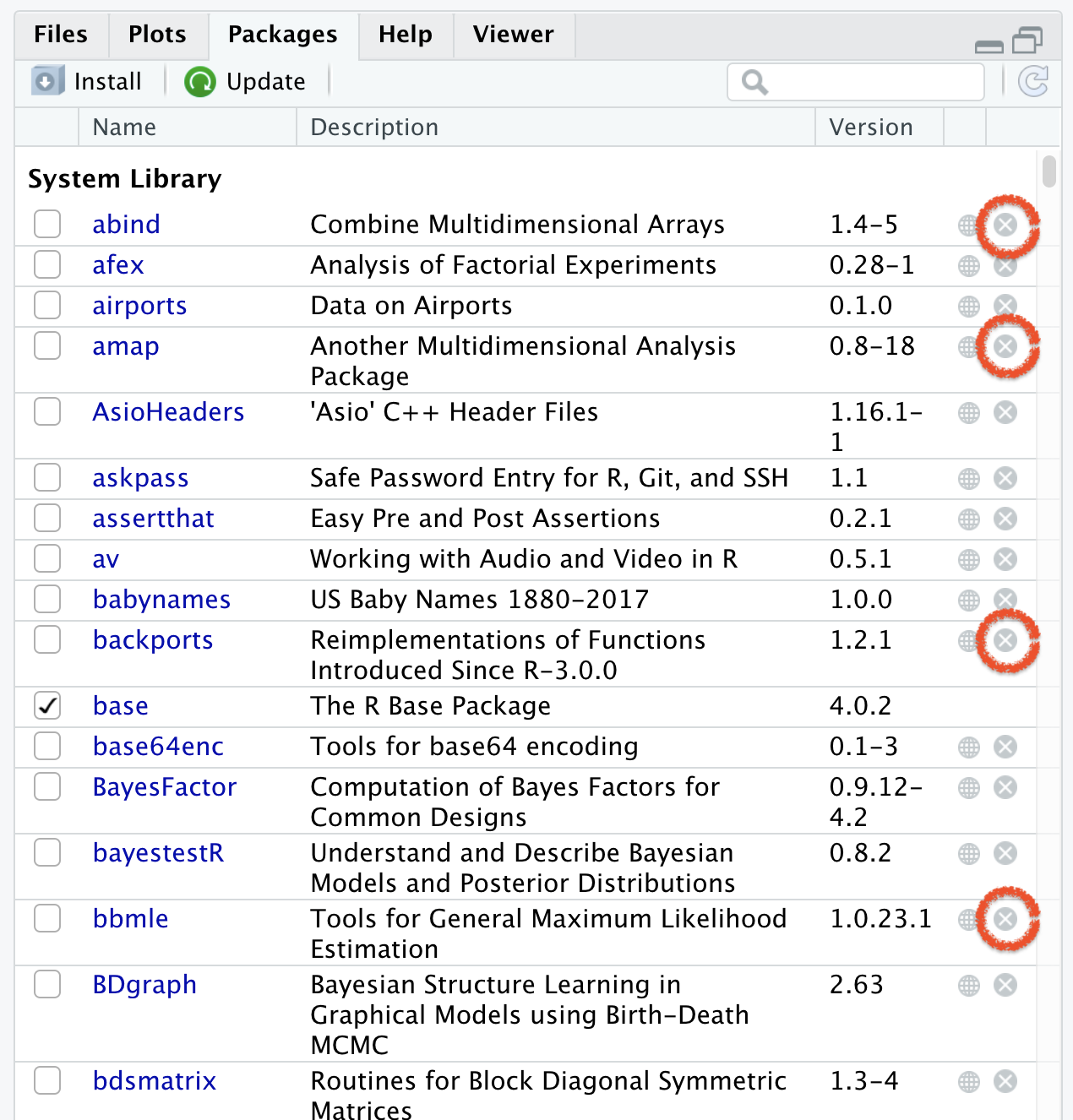
RStudio Environment Window
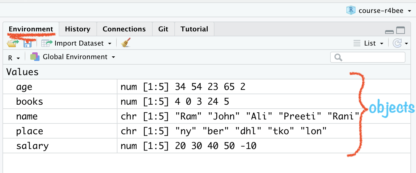
RStudio Environment Window
🤔how to combine these
objects/variables into a data or say tidy data
Tidy data 👇 😻😻😻
## age books name place salary## 1 34 4 Ram ny 20## 2 54 0 Rani ber 30## 3 23 3 Ali dhl 40## 4 65 24 Preeti tko 50## 5 2 5 John lon -10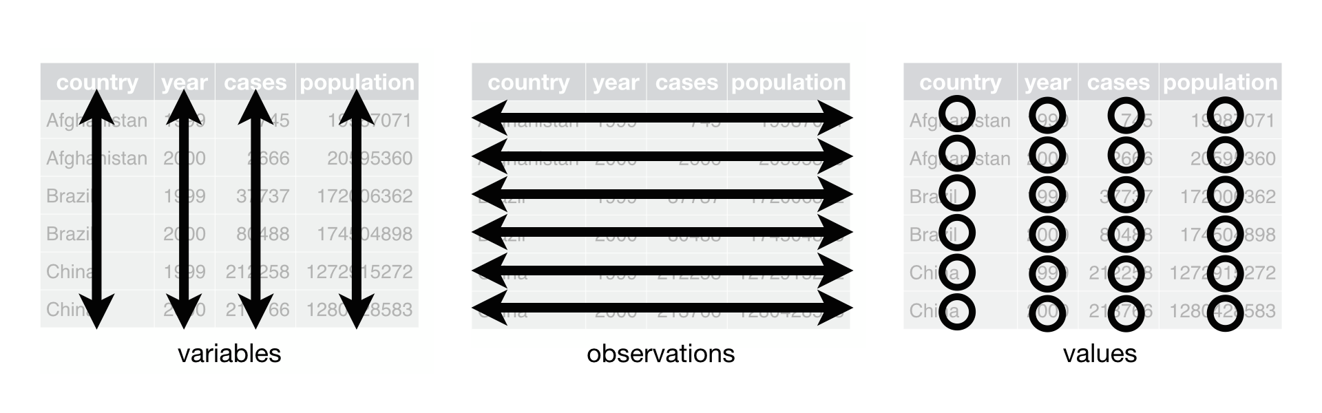
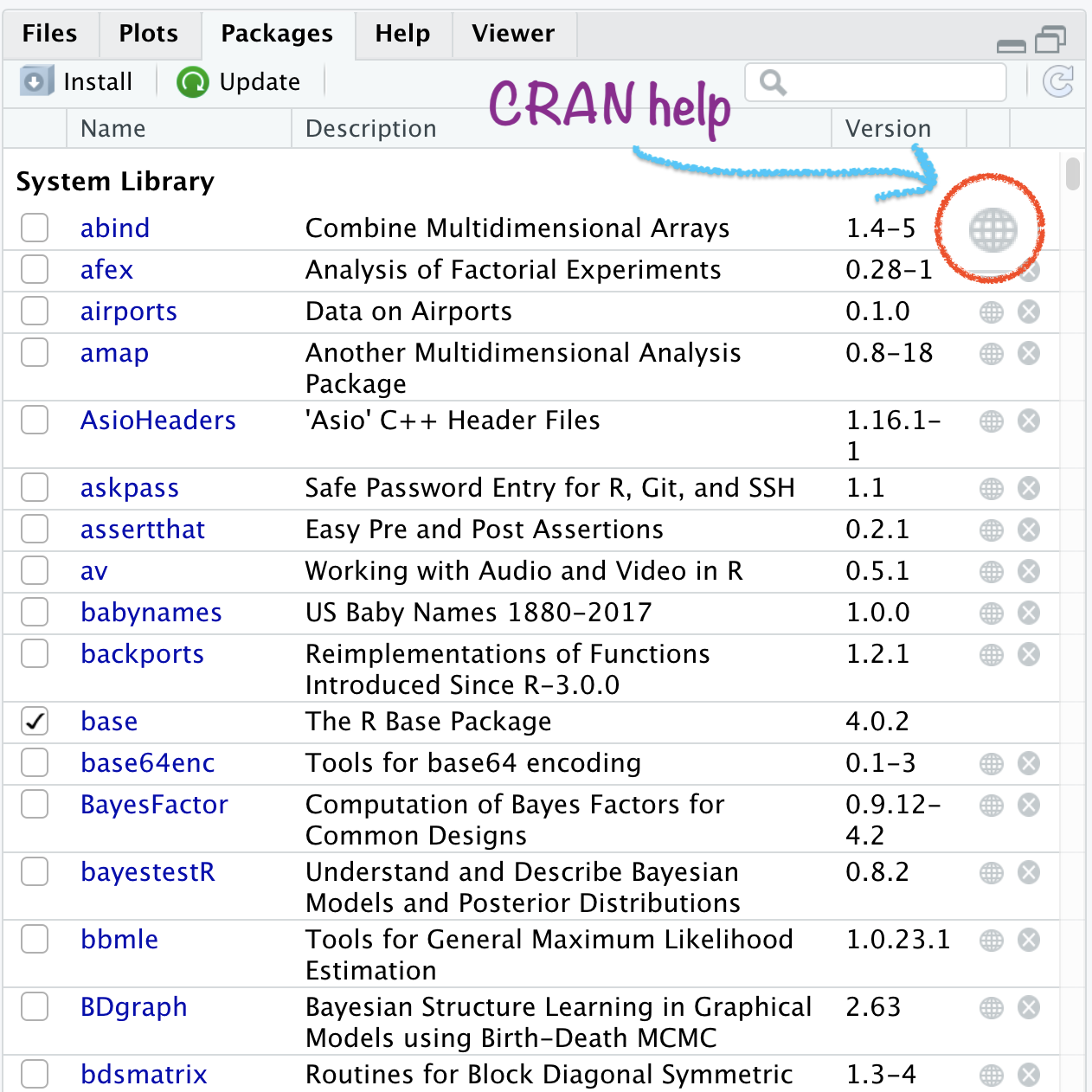
RStudio: pkg Help Docs
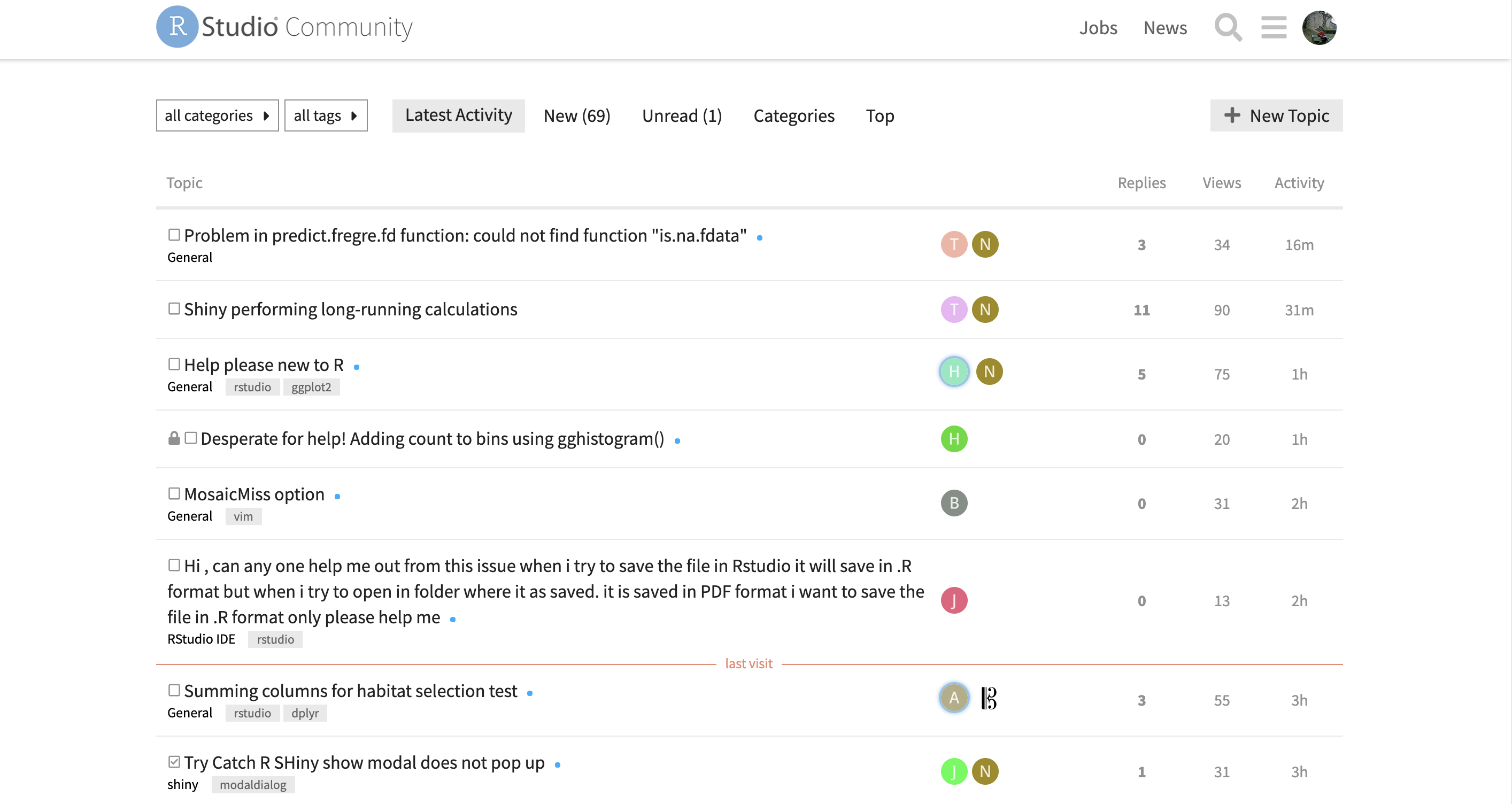
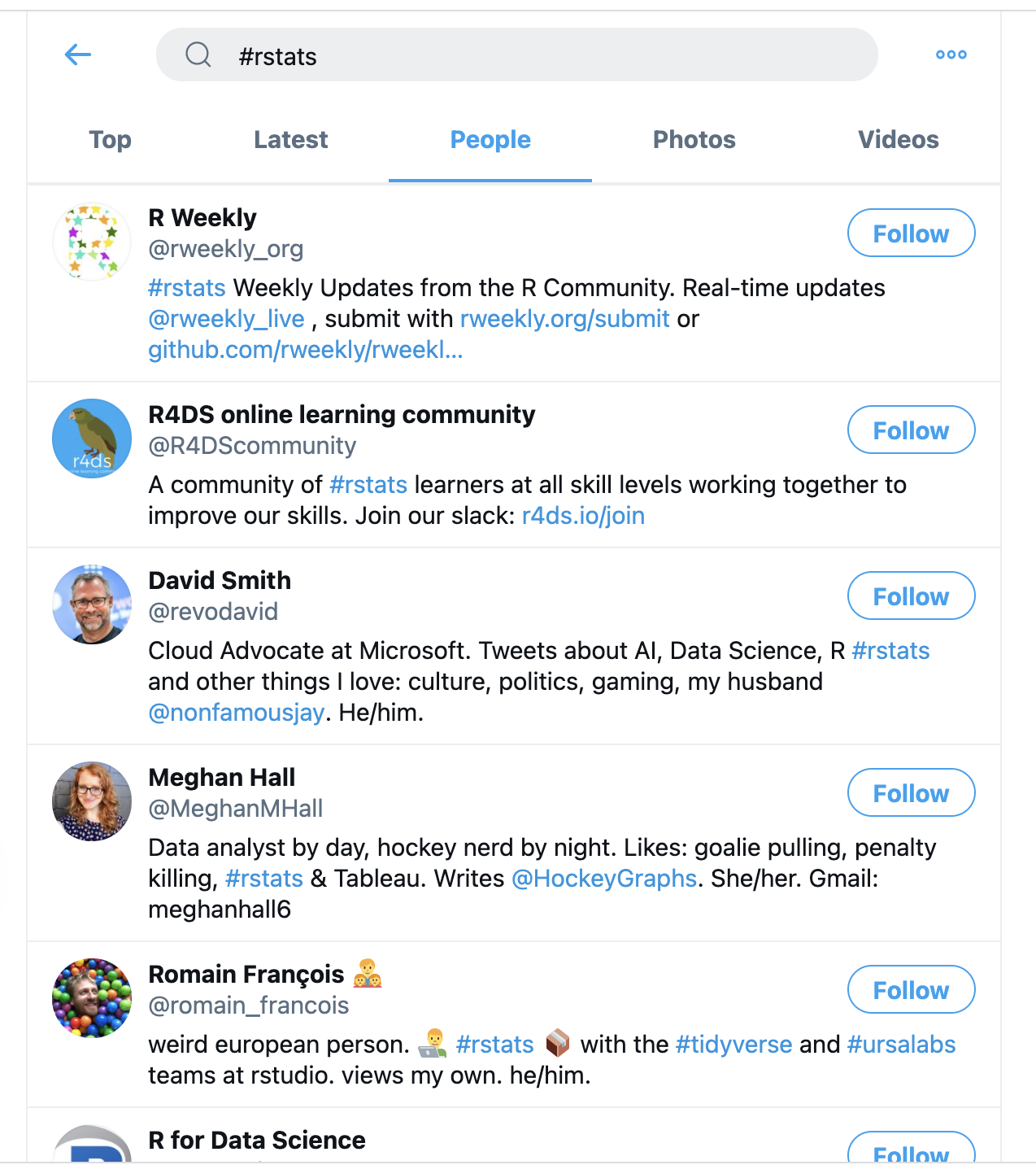
Twitter #rstats
Open RStudio
Open RStudio
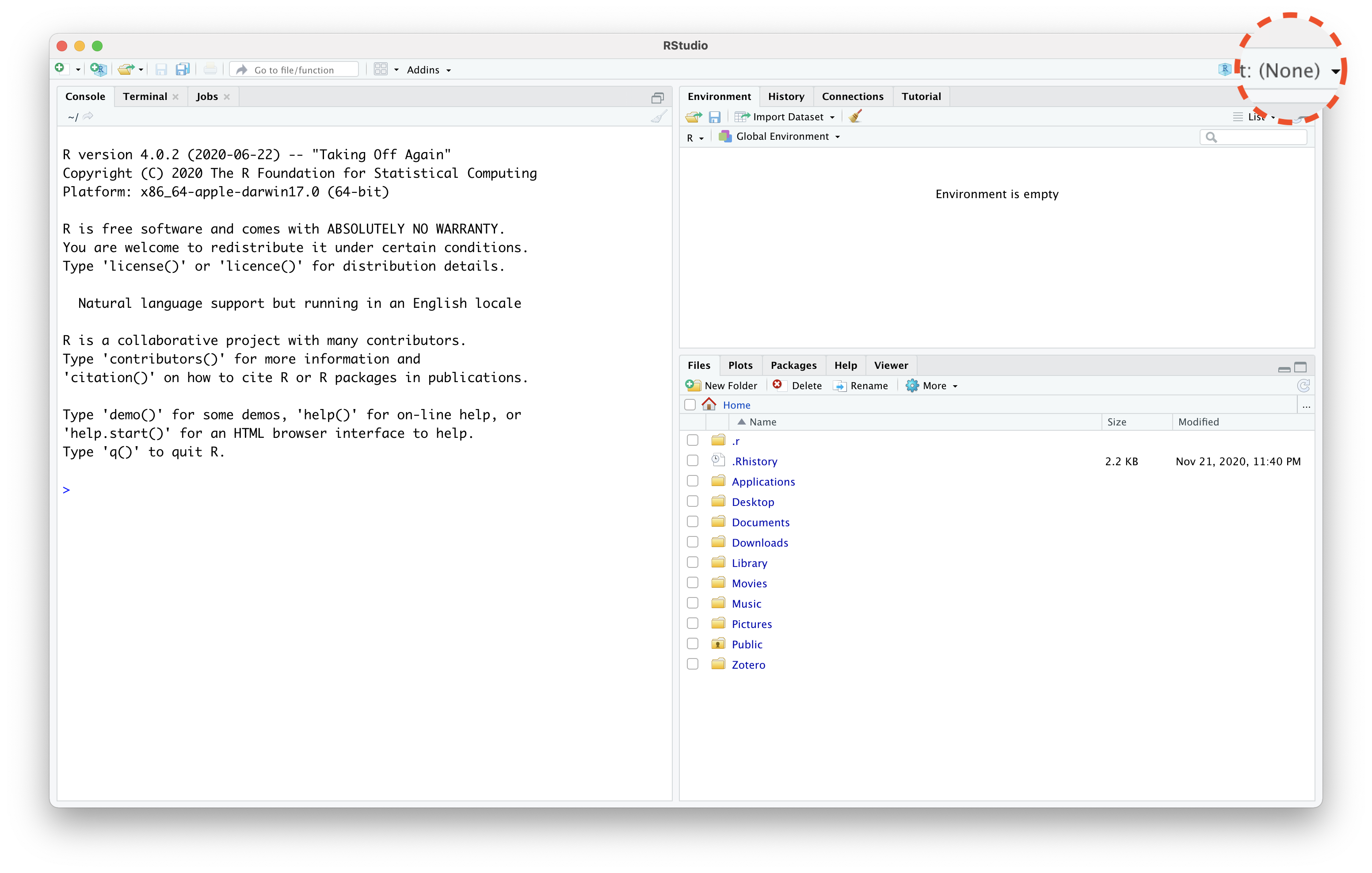
Open RStudio
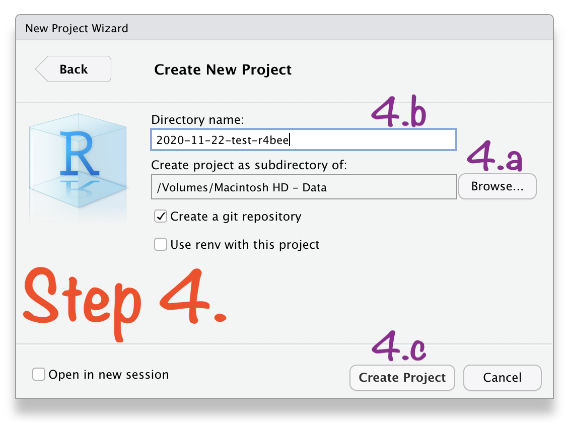
Create RStudio Project in 4 Steps
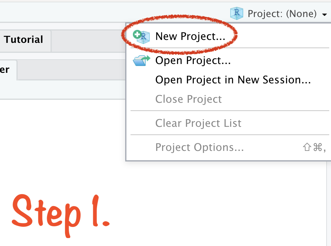
Create RStudio Project in 4 Steps
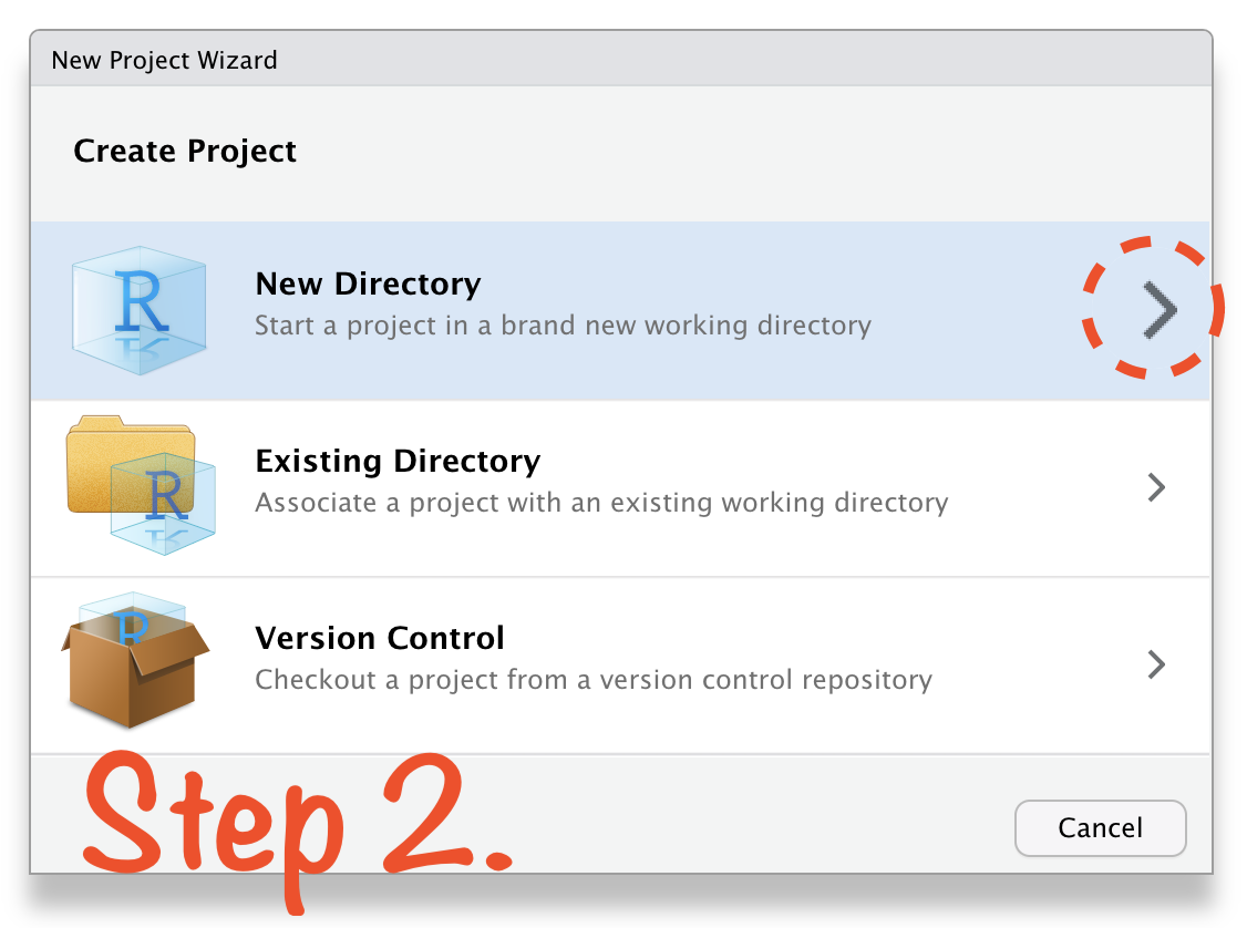
Create RStudio Project in 4 Steps
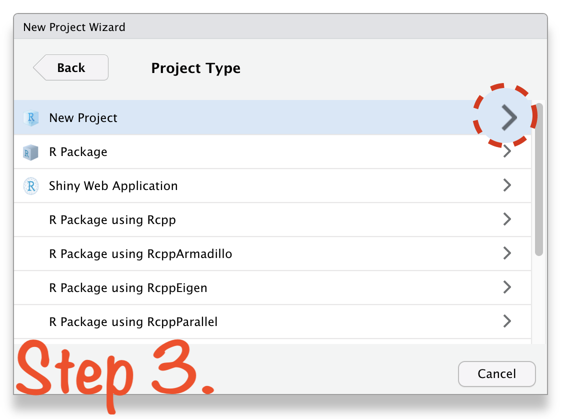
Create RStudio Project in 4 Steps
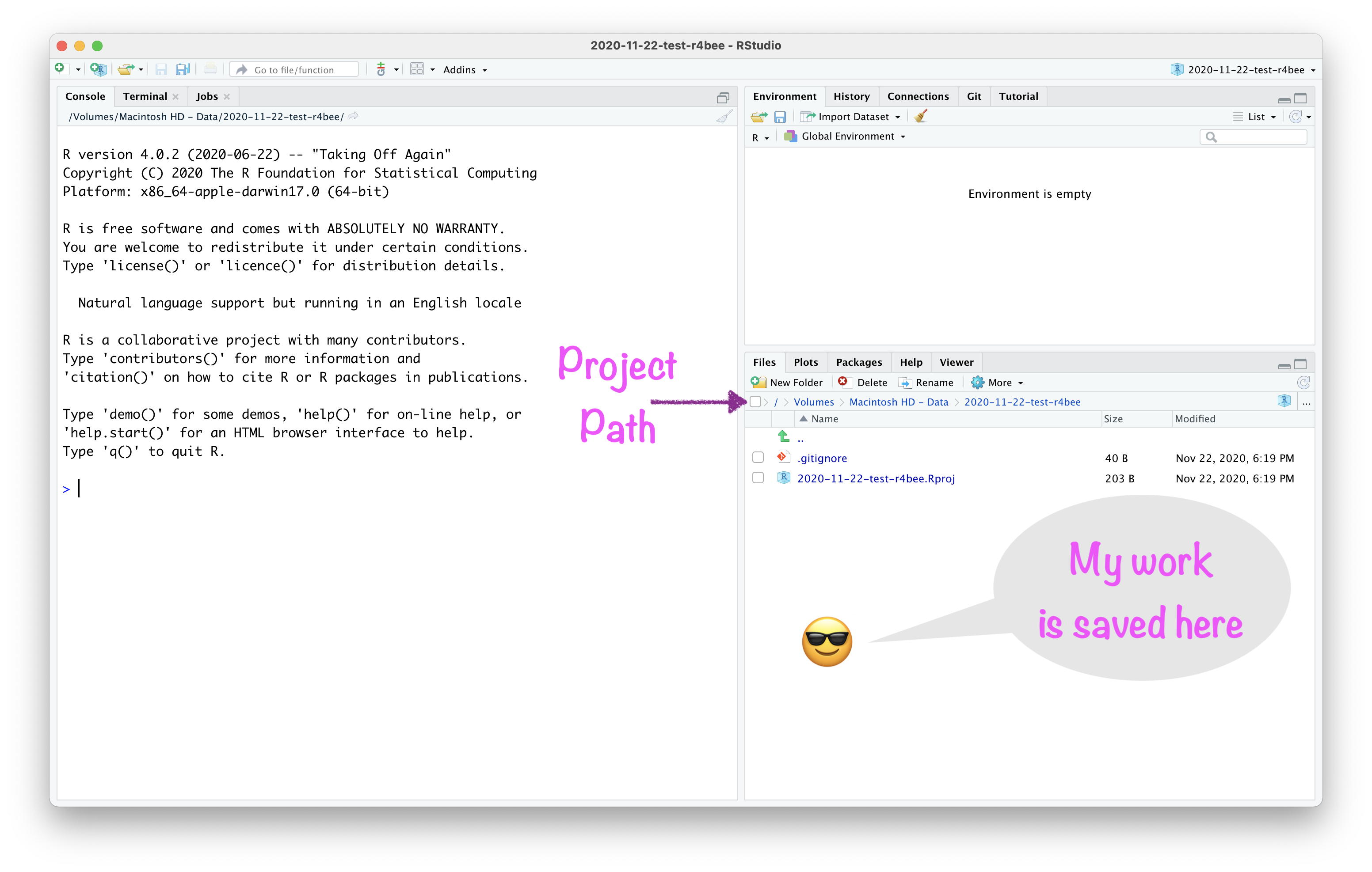
Open RStudio Project
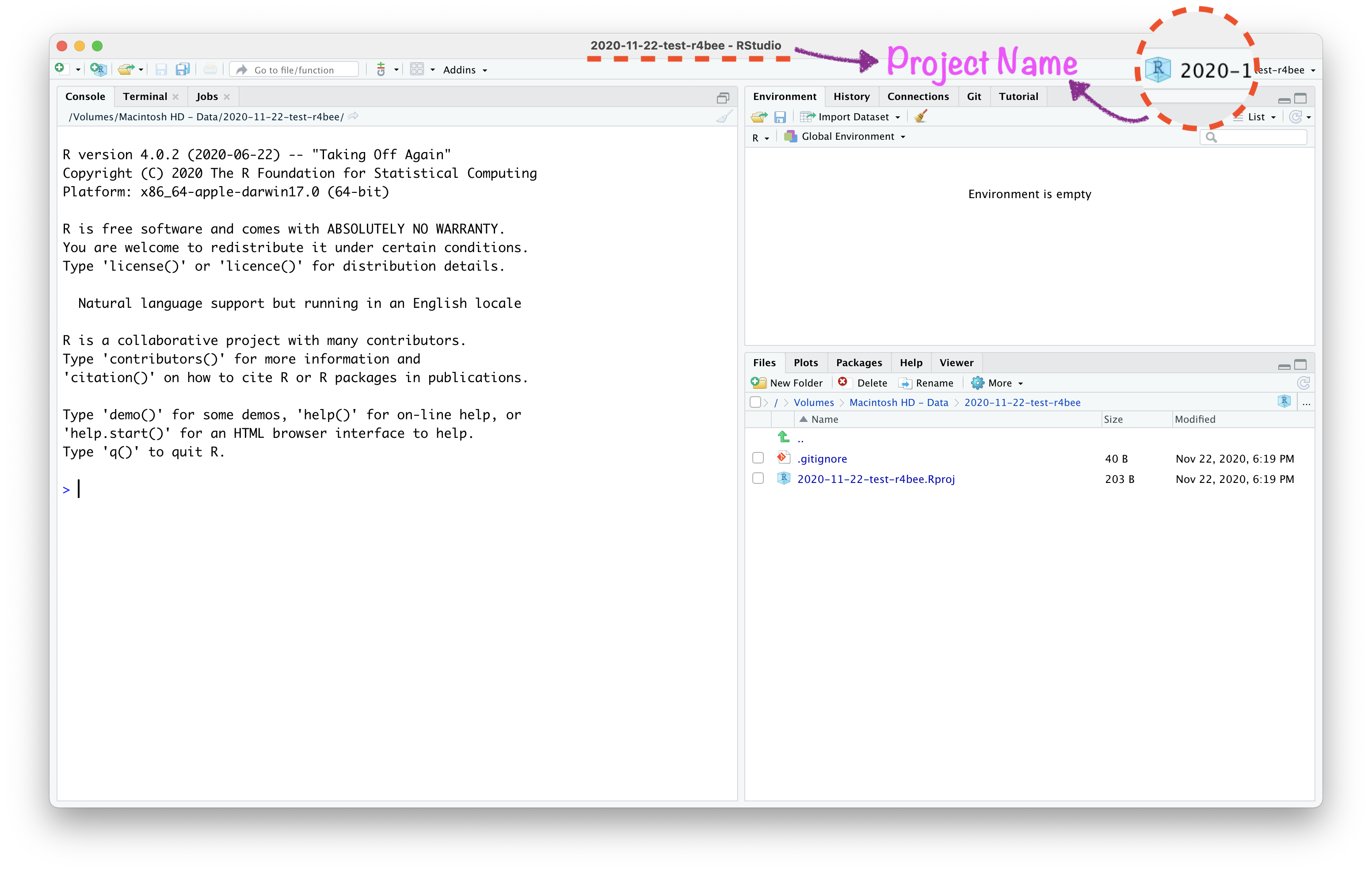
Open RStudio Project
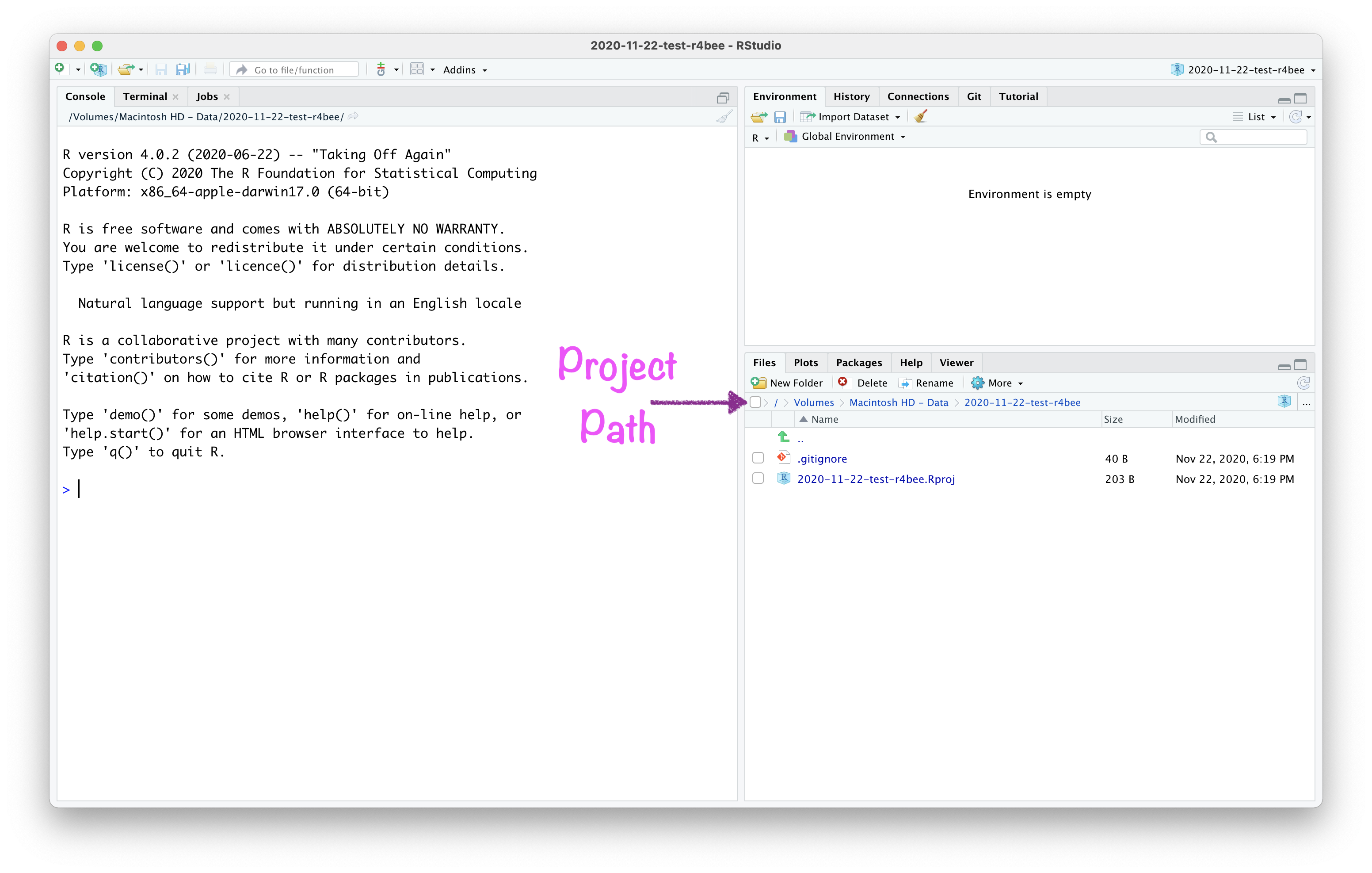
Open RStudio Project
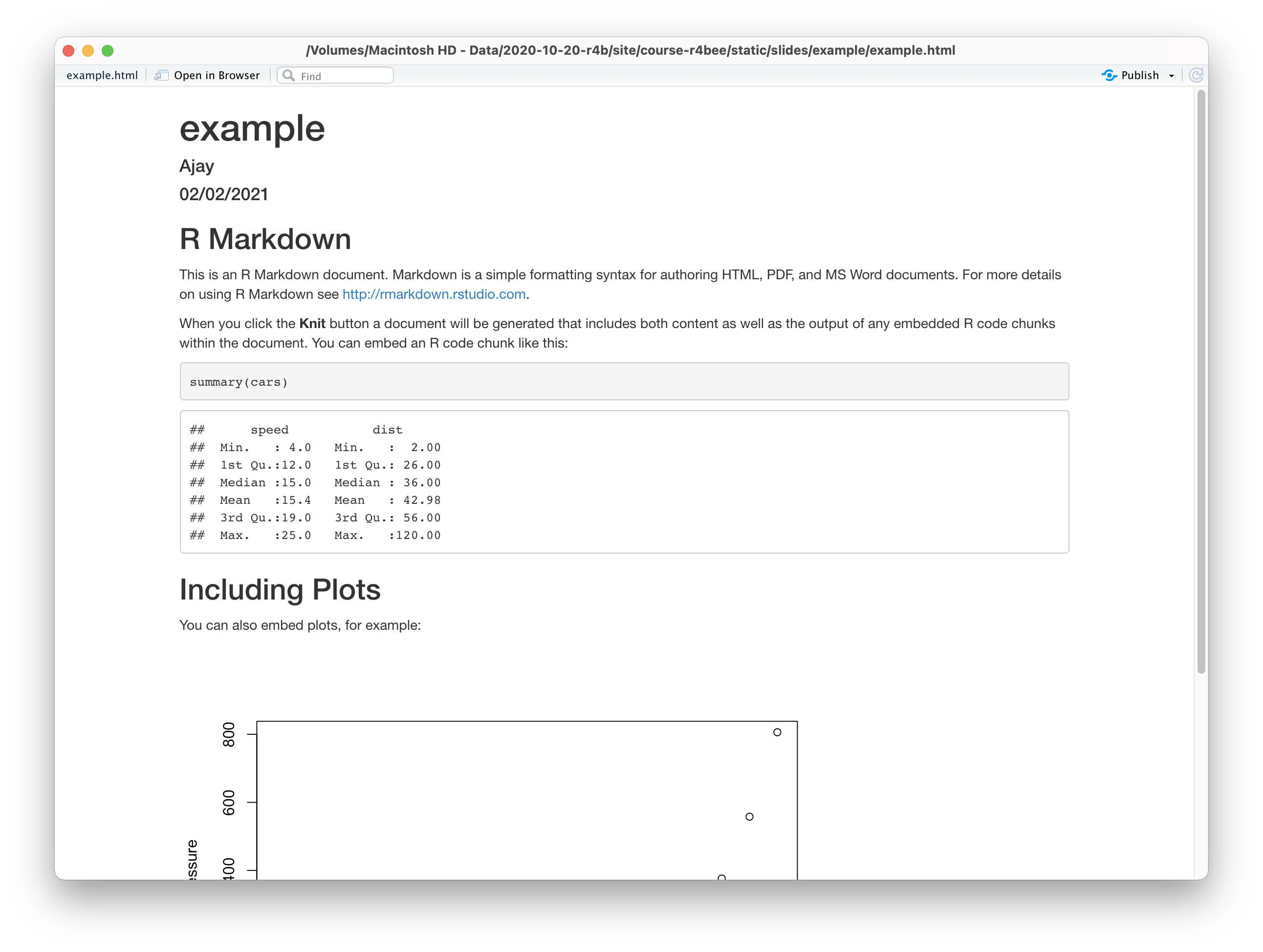
File \(\rightarrow\) New File \(\rightarrow\) R Markdown
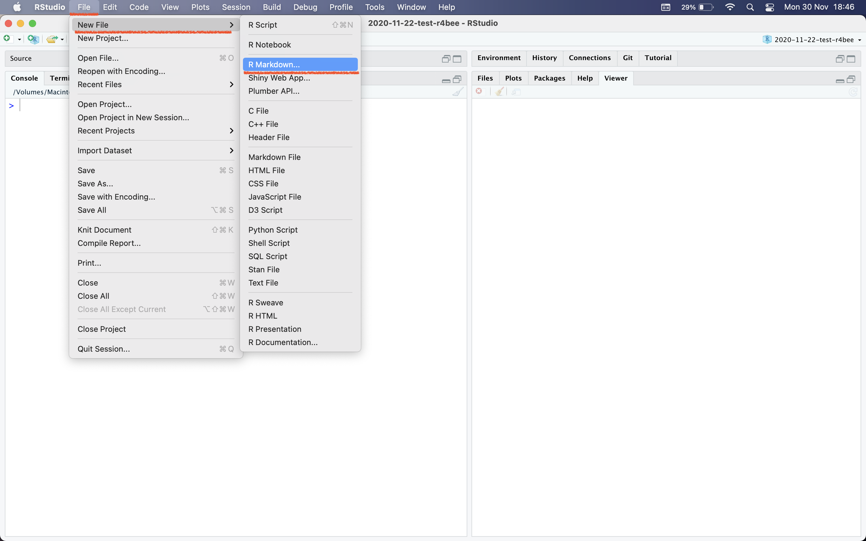
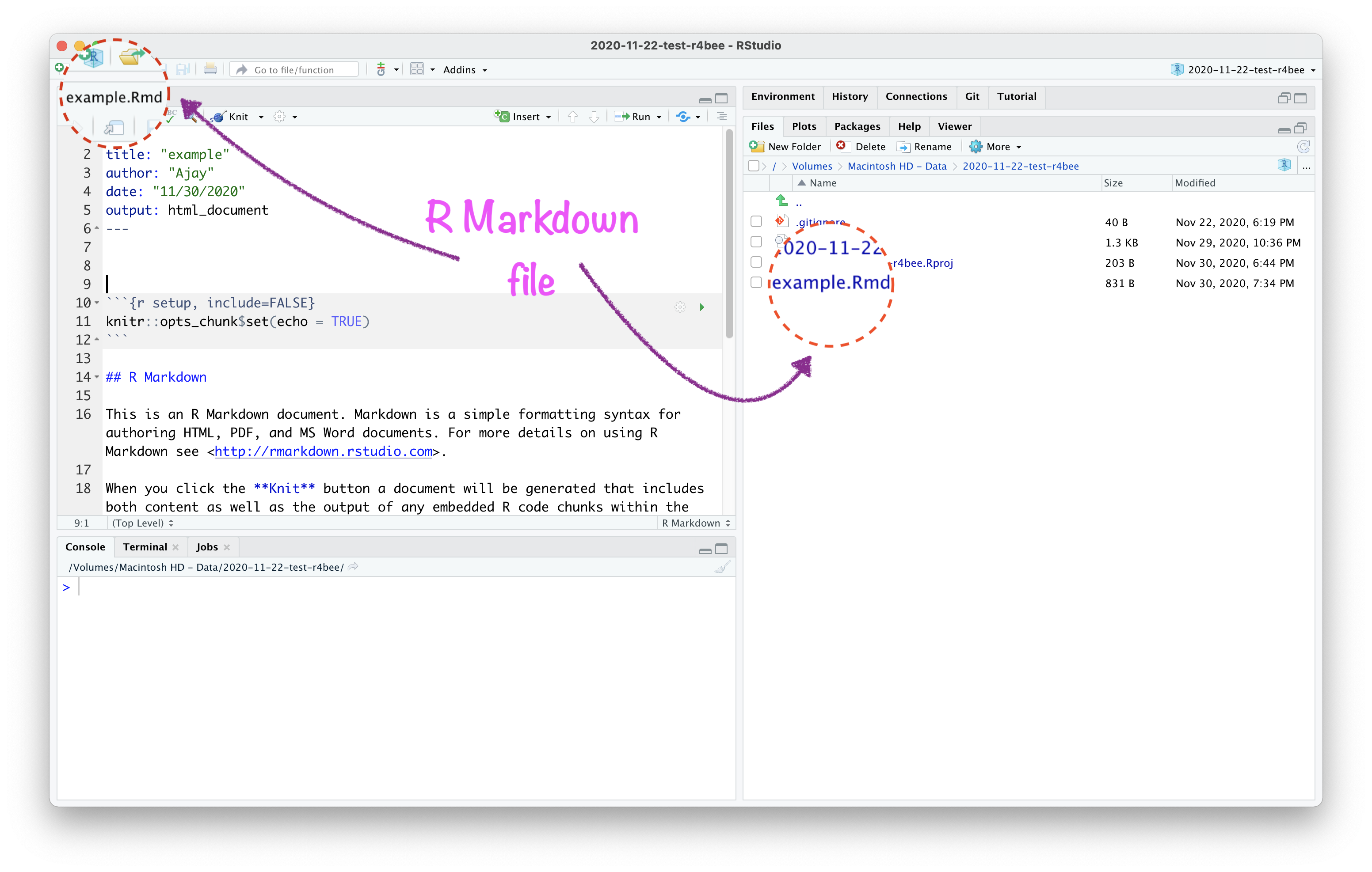
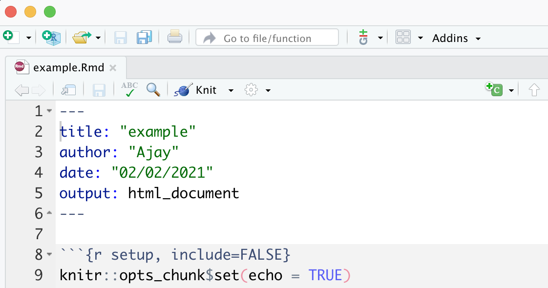
R Markdown
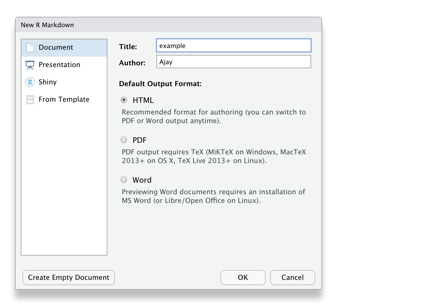
R Markdown
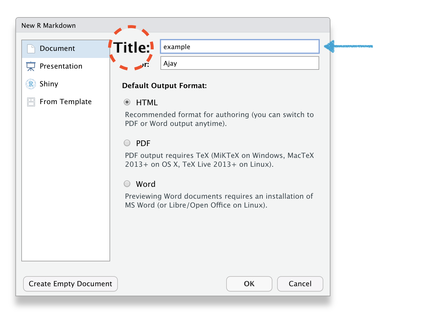
R Markdown
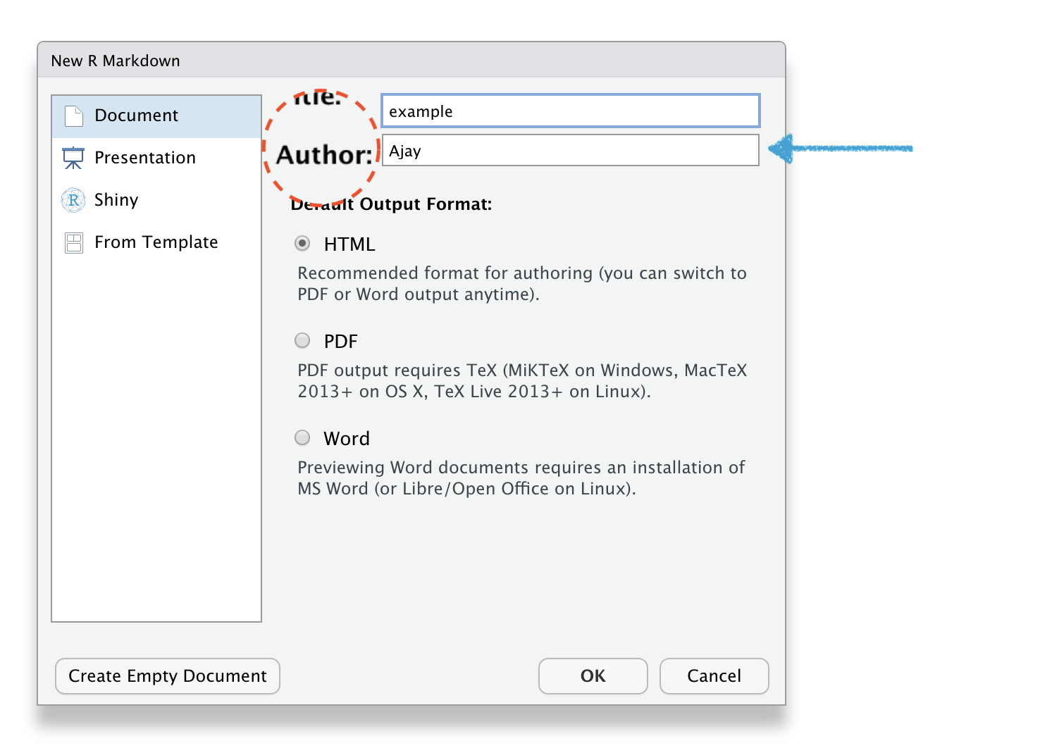
R Markdown

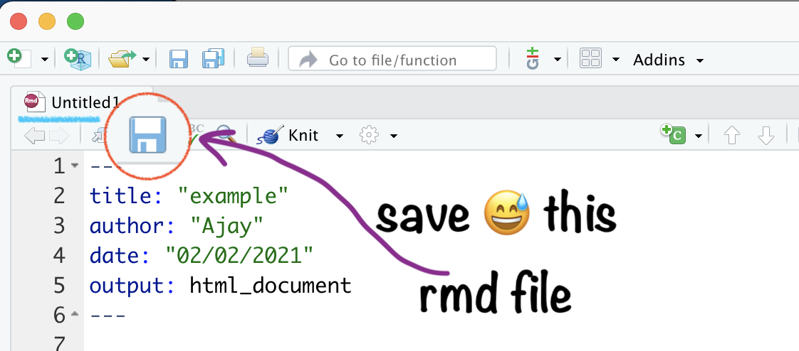
Save your .Rmd file
Name your .Rmd file
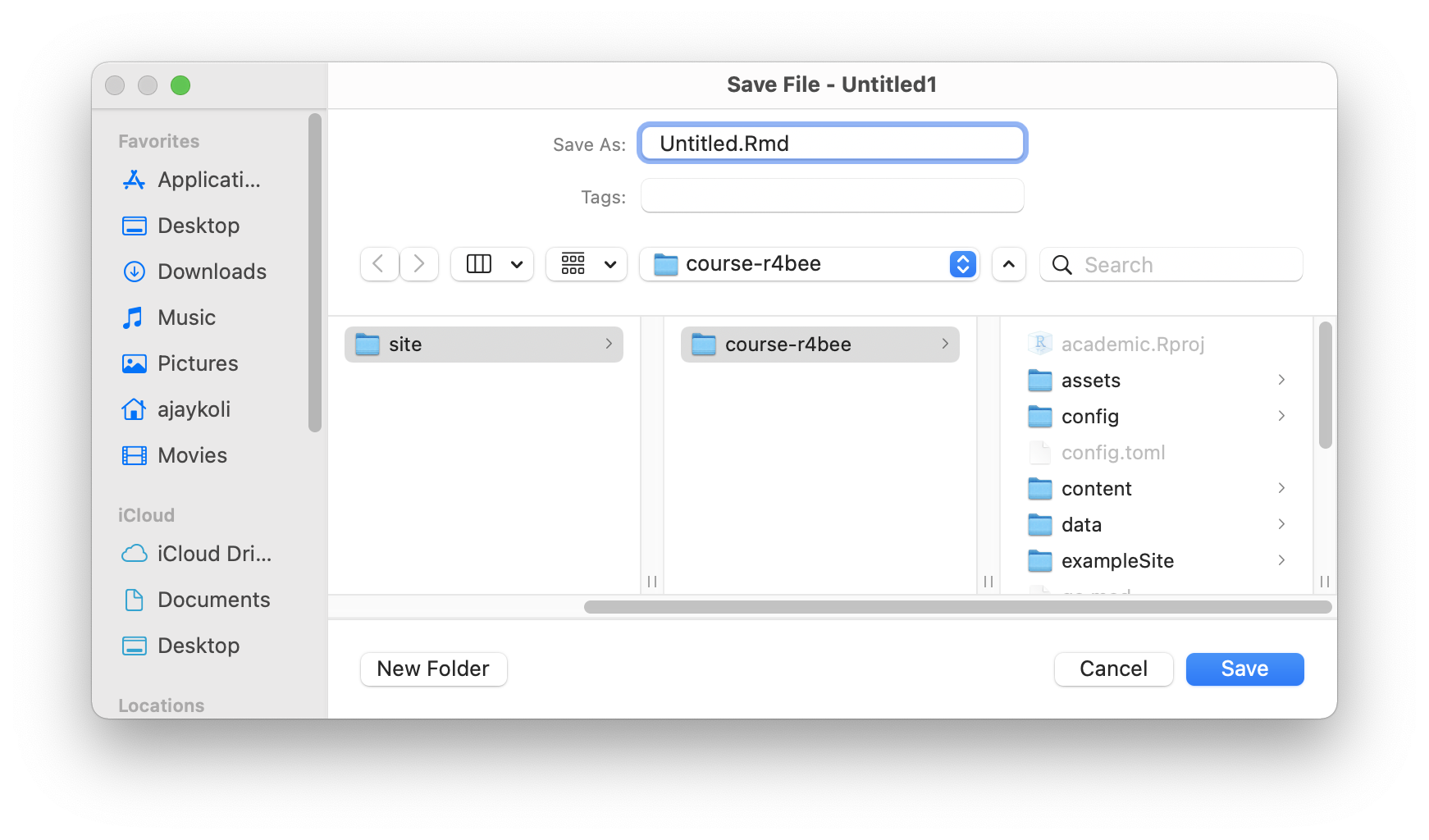
Name your .Rmd file
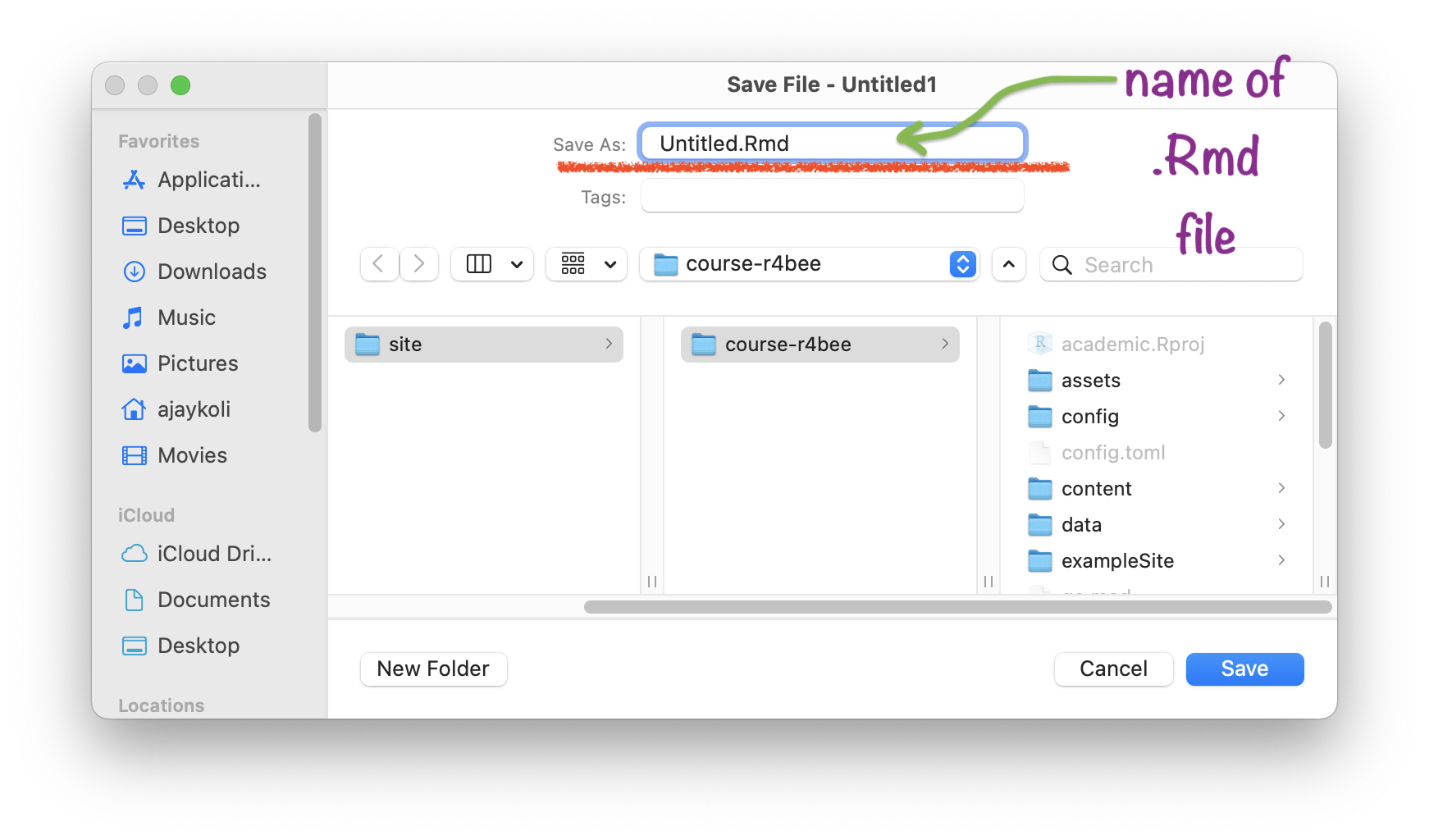
Save your .Rmd file
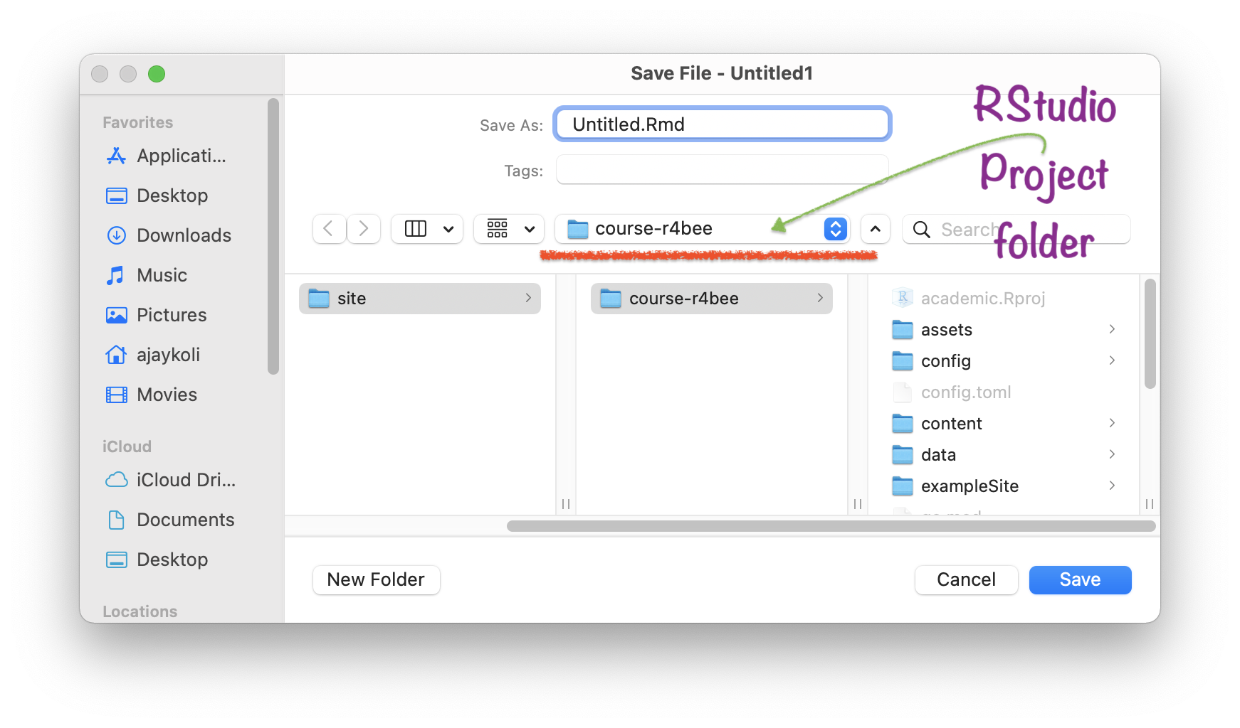
Saved .Rmd file \(\rightarrow\) in RStudio Project
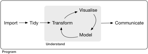
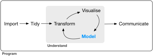
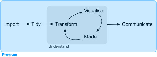
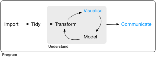
Course Progress
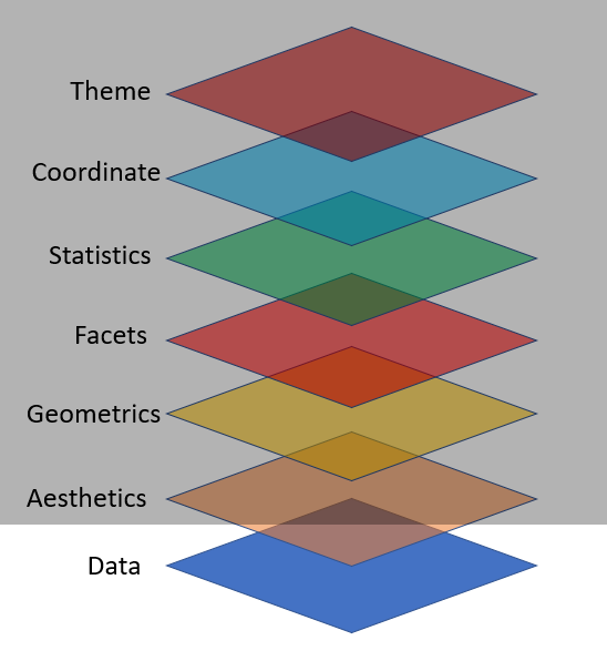
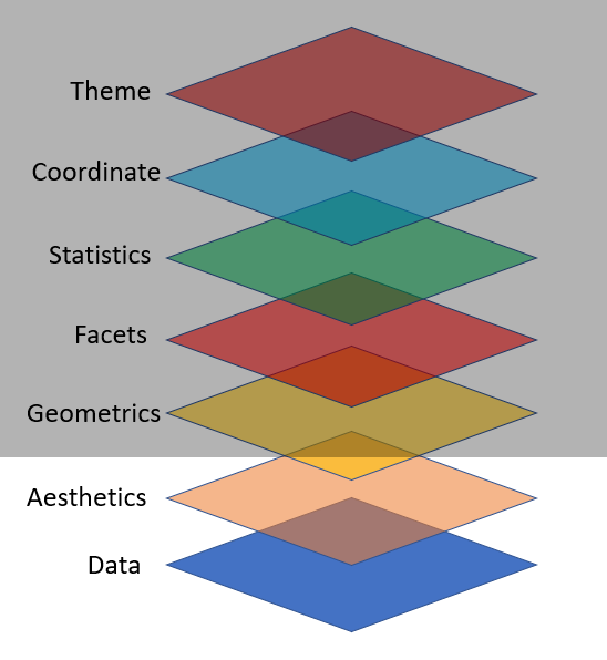
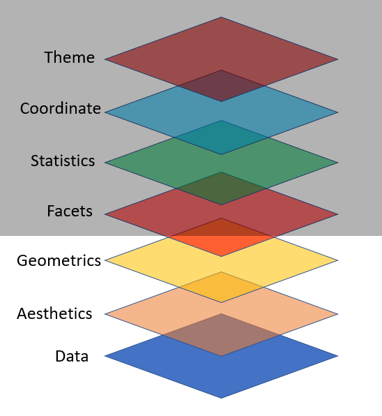
ggplot2 by Hadley Wickham
- "is a system for declaratively creating graphics, based on The Grammar of Graphics" (book by Late Leland Wilkinson)

Late Leland Wilkinson

Hadley Wickham


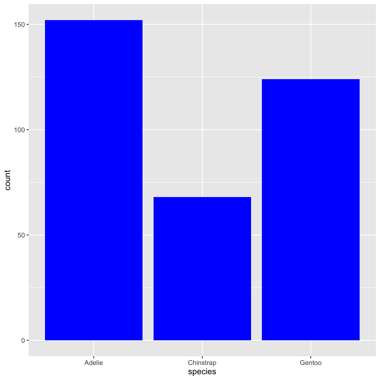
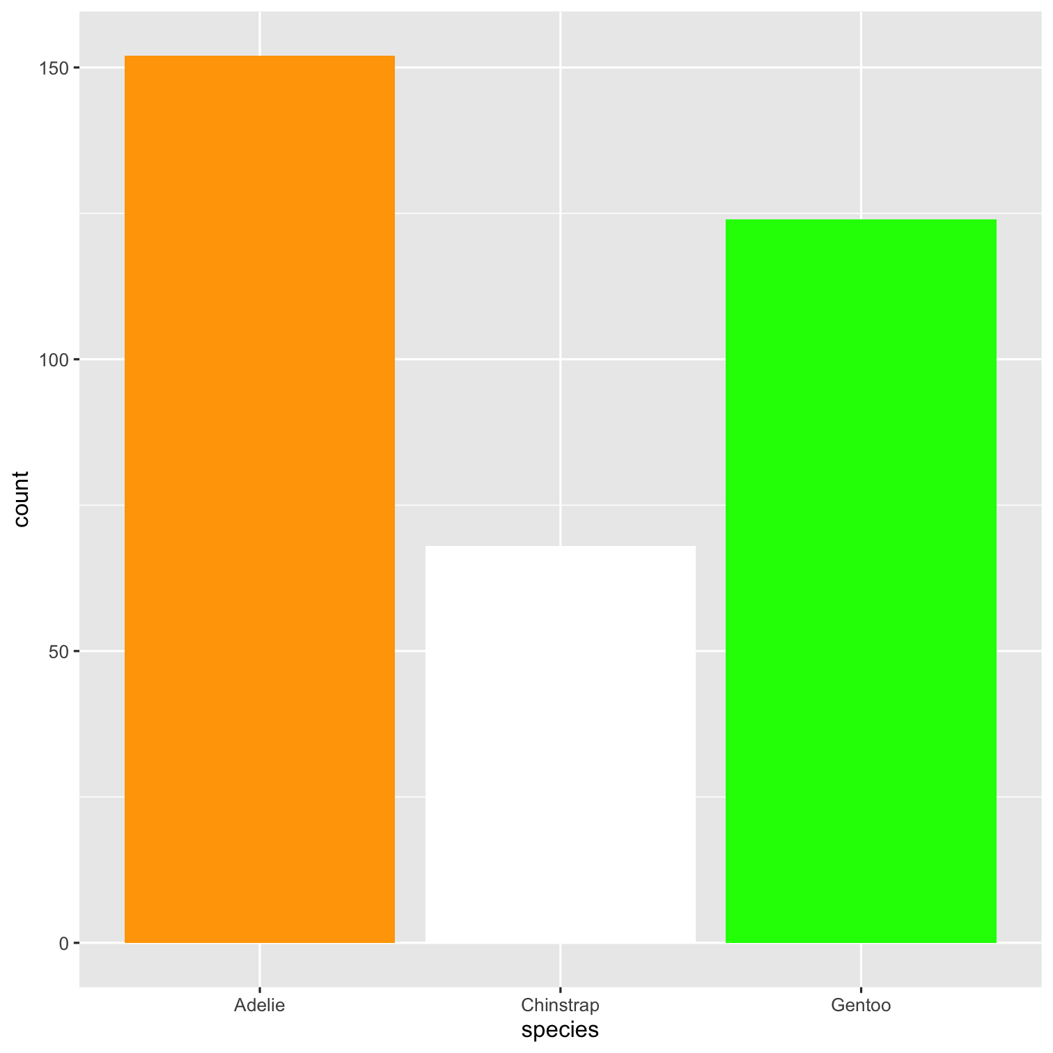
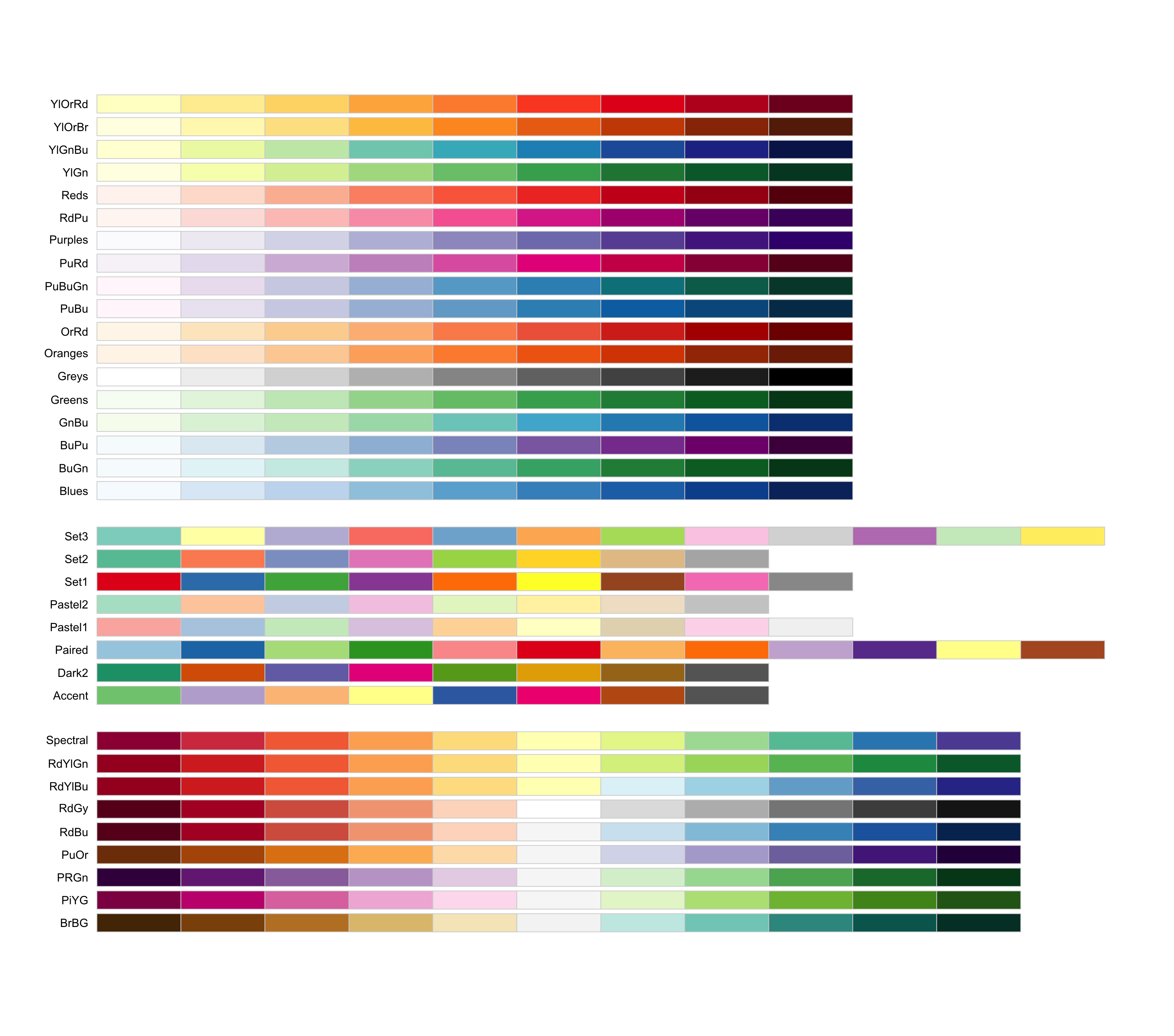
🎨 Color Palette
- R package
RColorBrewer&wesanderson
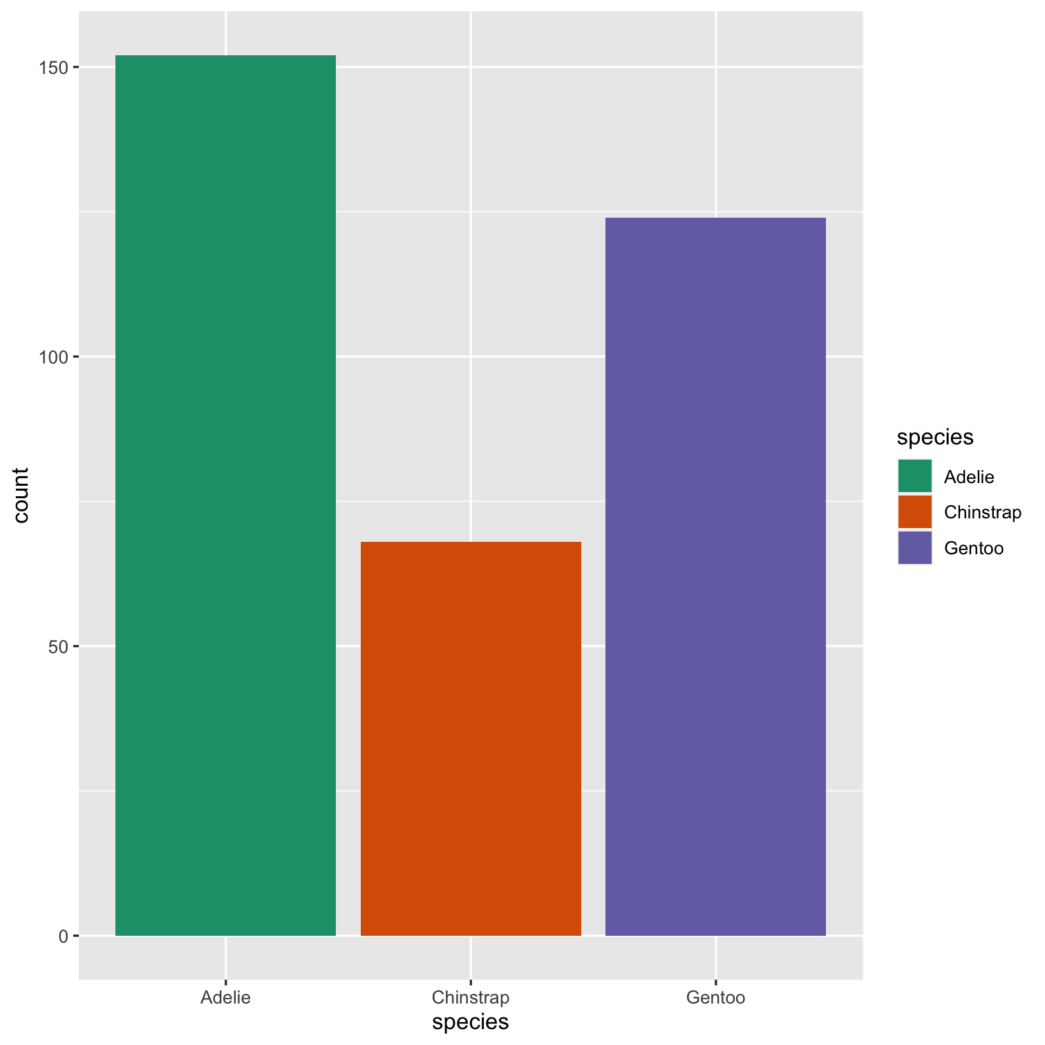
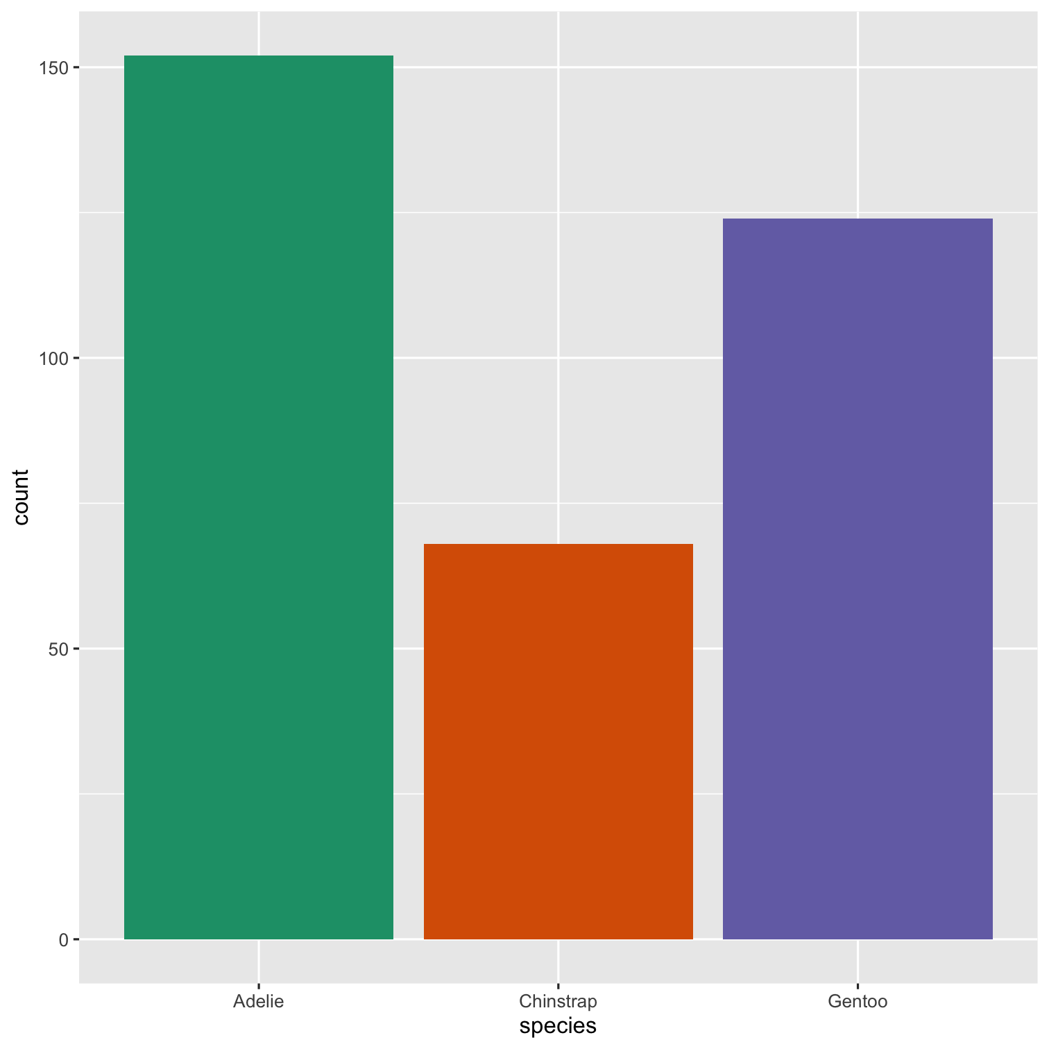
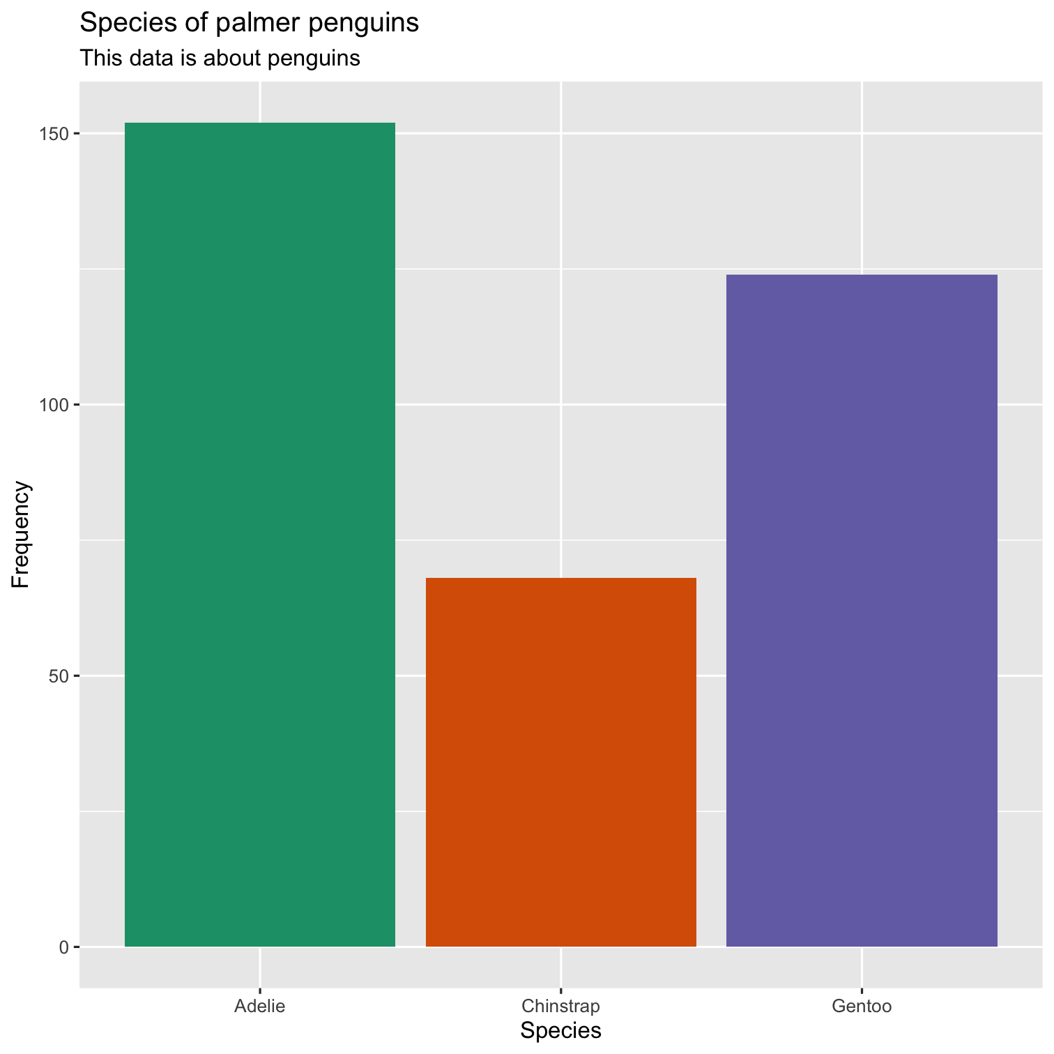
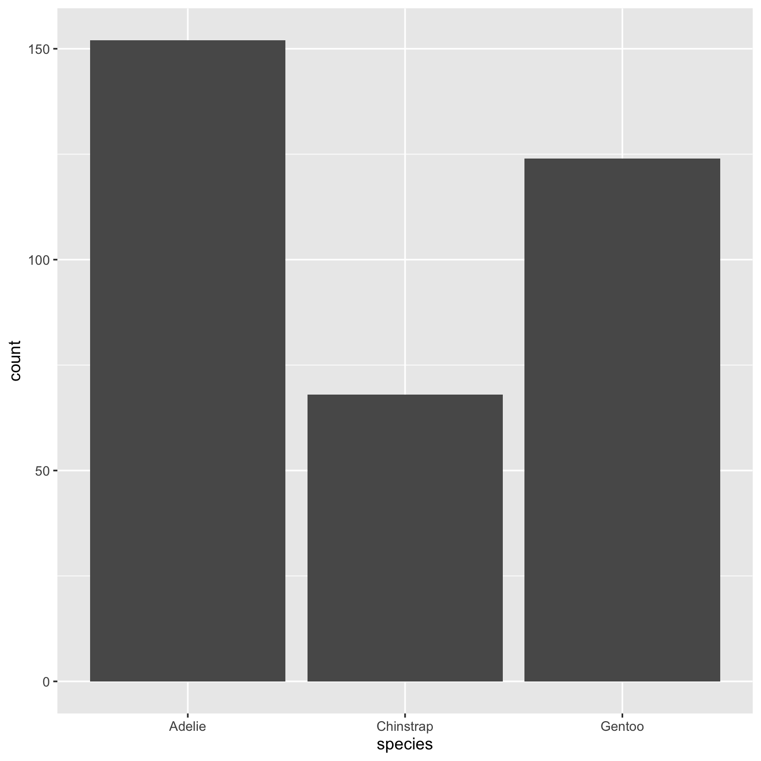
ggplot(data = penguins, mapping = aes(x = species, fill = species)) + geom_bar() + scale_fill_brewer(palette = "Dark2") + theme(legend.position = "none", text = element_text(size = 20)) + labs( title = "Species of palmer penguins", subtitle = "This data is about penguins", x = "Species", y = "Frequency" )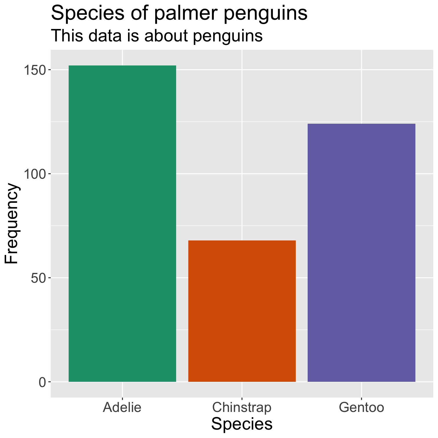
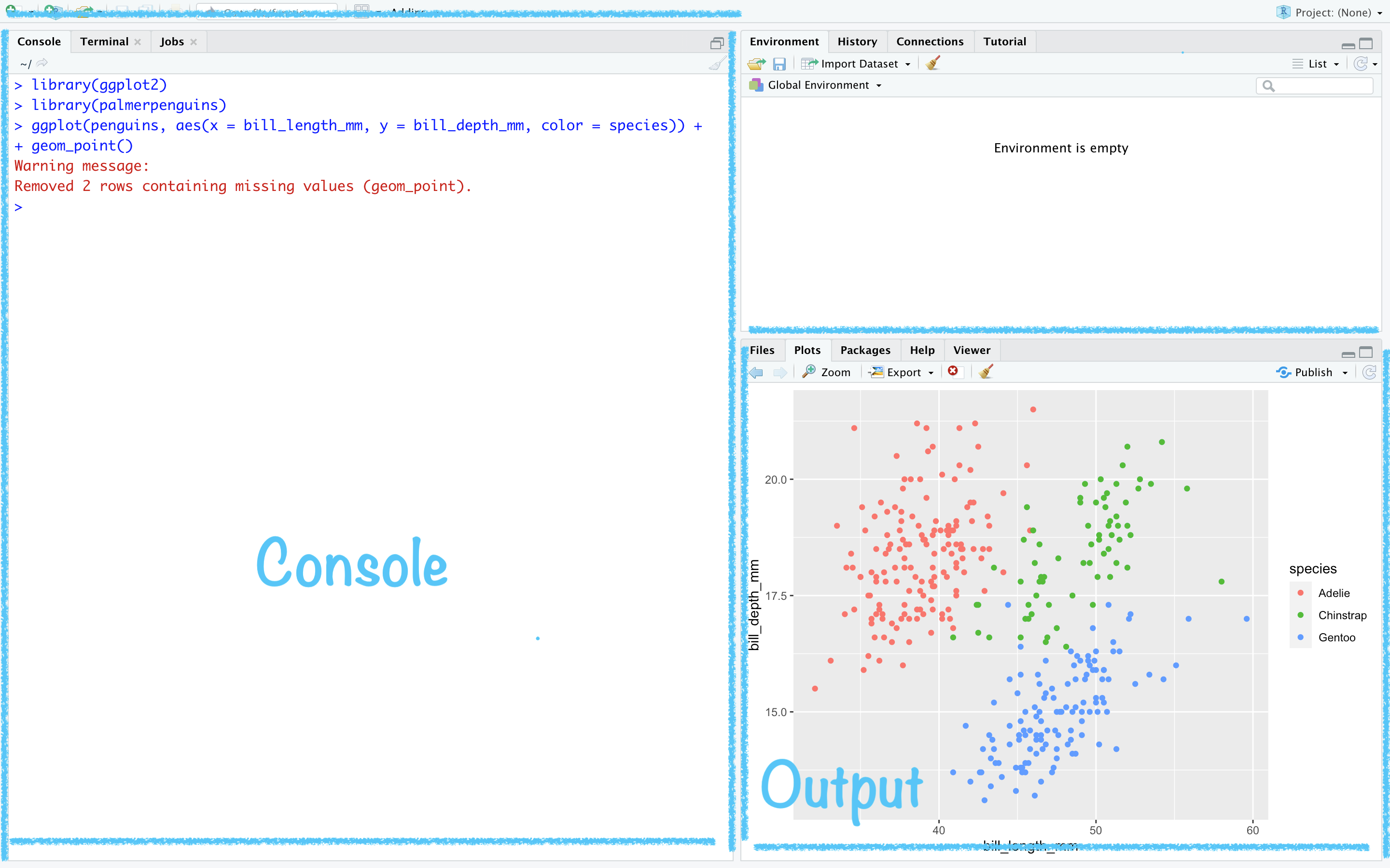
ggplot(data = penguins, mapping = aes(x = bill_length_mm, y = bill_depth_mm, color = species)) + geom_point() + scale_fill_brewer(palette = "Dark2") + theme(legend.position = "none", text = element_text(size = 20)) + labs( title = "Relationship between bill length \n& depth of palmer penguins", subtitle = "This data is about penguins", x = "Bill length (mm)", y = "Bith depth (mm)" )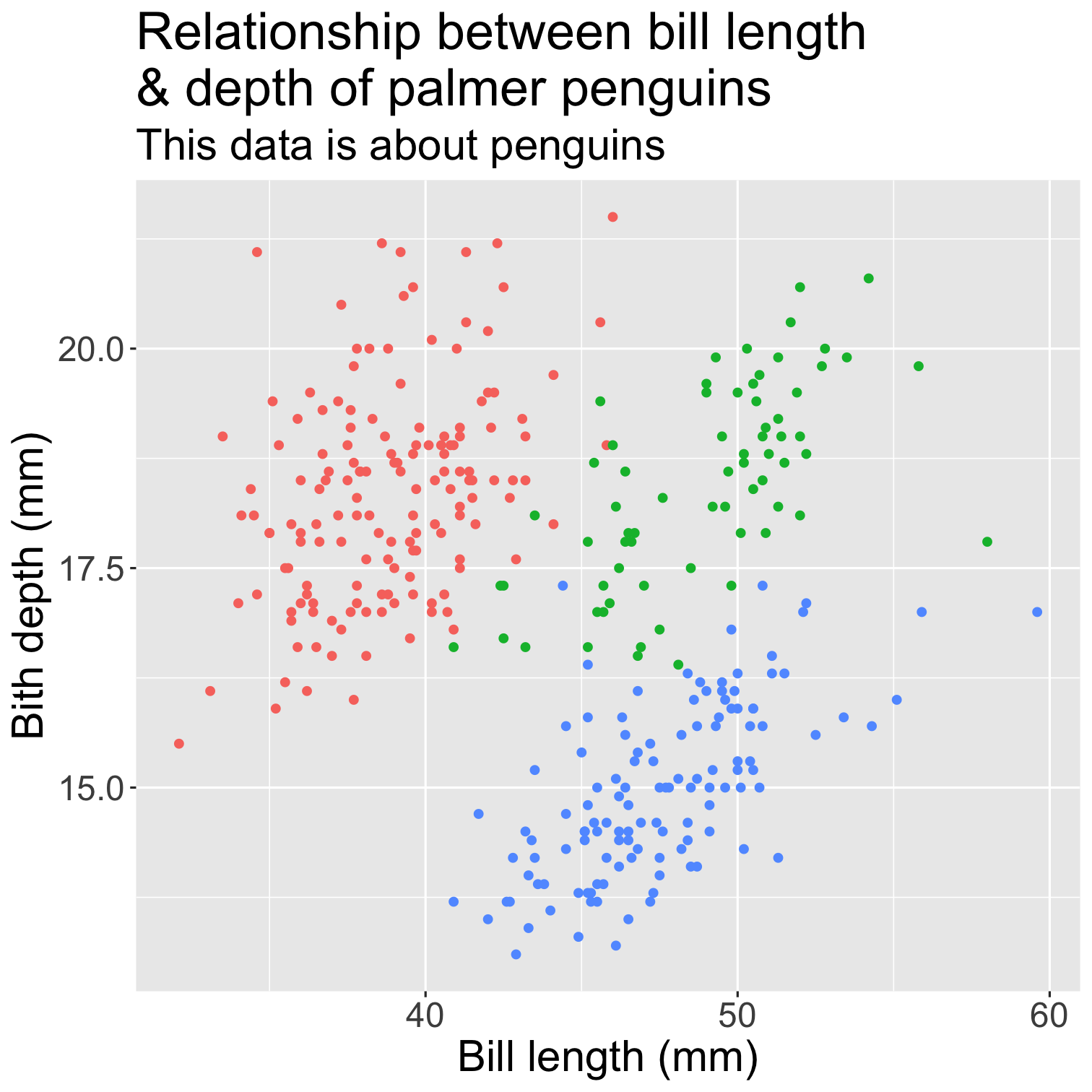
ggplot(data = penguins, mapping = aes(x = bill_length_mm, y = bill_depth_mm, color = species)) + geom_point() + scale_fill_brewer(palette = "Dark2") + theme(legend.position = "none", text = element_text(size = 20)) + labs( title = "Relationship between bill length \n& depth of palmer penguins", subtitle = "This data is about penguins", x = "Bill length (mm)", y = "Bith depth (mm)" ) + theme_bw()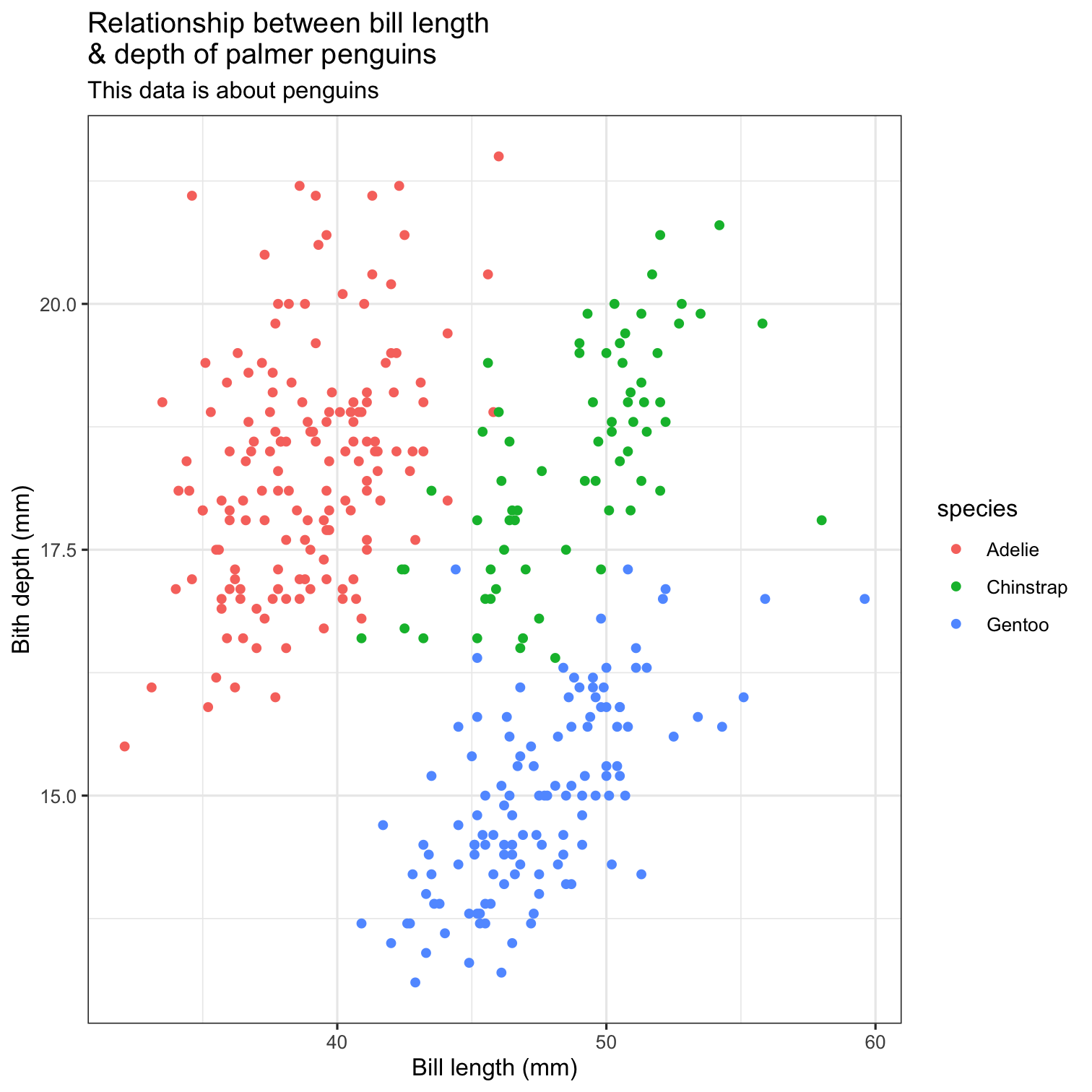
ggplot(data = penguins, mapping = aes(x = bill_length_mm, y = bill_depth_mm, color = species)) + geom_point() + scale_fill_brewer(palette = "Dark2") + theme(legend.position = "none", text = element_text(size = 20)) + labs( title = "Relationship between bill length \n& depth of palmer penguins", subtitle = "This data is about penguins", x = "Bill length (mm)", y = "Bith depth (mm)" ) + theme_classic()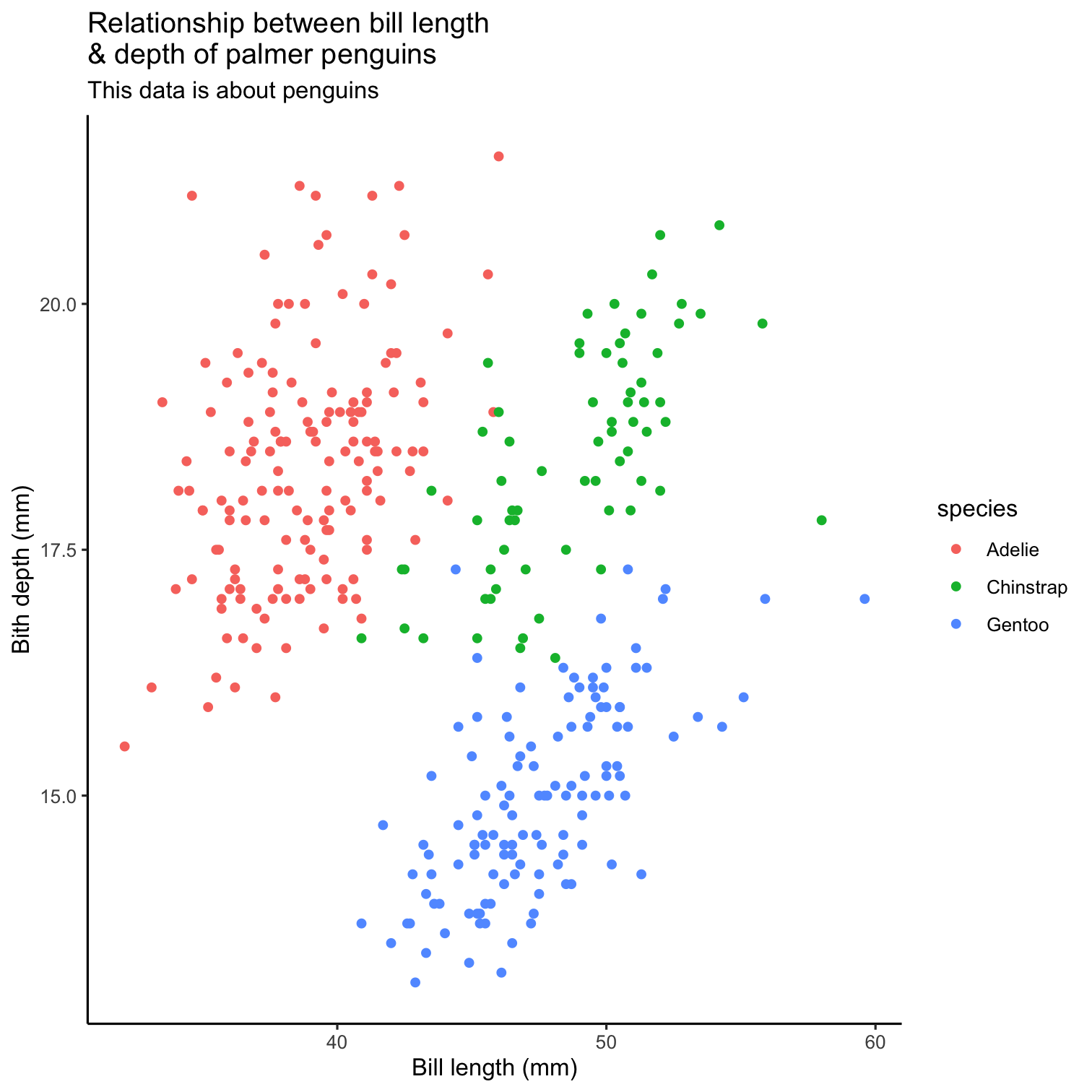
ggplot(data = penguins, mapping = aes(x = flipper_length_mm, y = body_mass_g)) + geom_point() + theme(legend.position = "none", text = element_text(size = 24)) + labs( title = "Relationship between bill length \n& depth of palmer penguins", subtitle = "This data is about penguins", x = "Flipper length (mm)", y = "Body mass (gm)" ) + theme_classic() + geom_smooth()
Course Progress
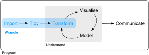
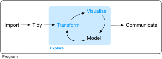
What is Data wrangling?
"data exploration and data manipulation" (Jesse Mostipak)
"tidying and transforming" (Hadley & Garrett)
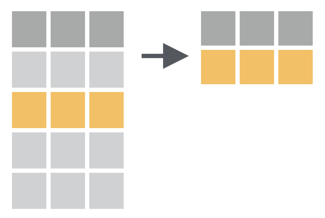
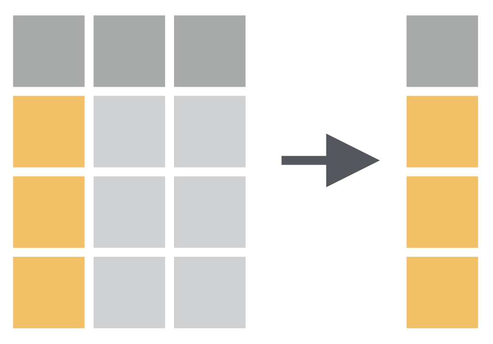
filter() function:
- Picks cases based on their values.
select() function: Chooses rows based on column values.
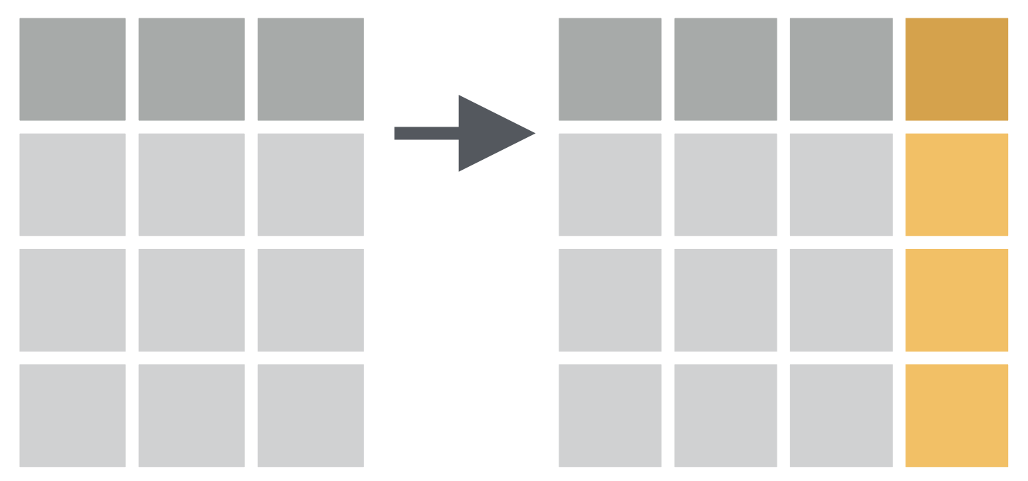
mutate() function: Adds new variables that are functions of existing variables
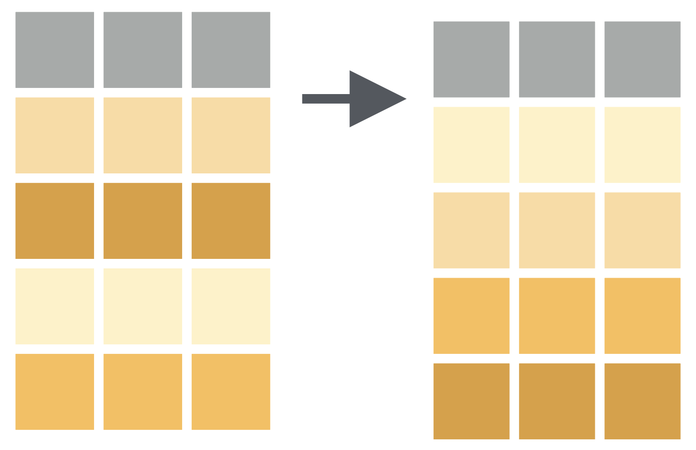
arrange() function: Changes the order of the rows.
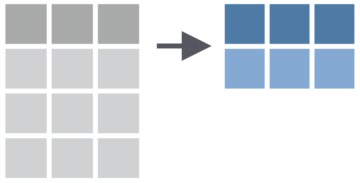
summarise() function: Chooses rows based on column values.
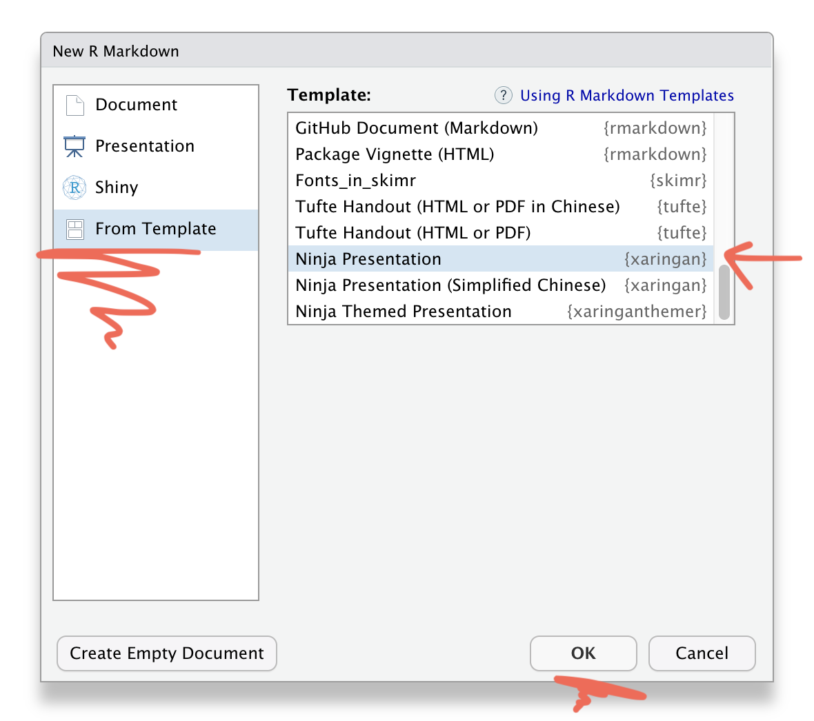
File \(\longrightarrow\) New File \(\longrightarrow\) R Markdown

Template \(\rightarrow\) Ninja Presentation
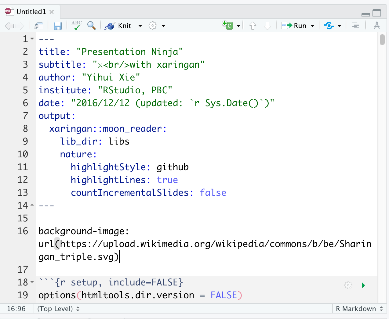
Save this Rmd file
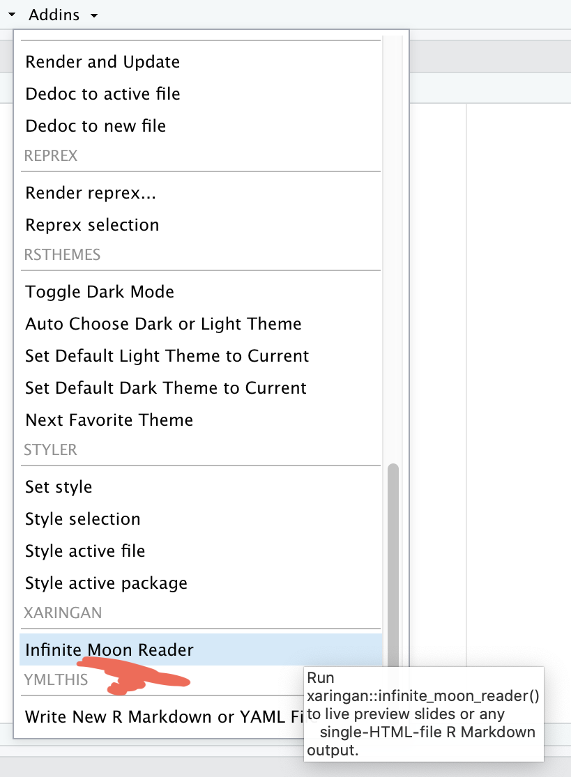
Addins \(\rightarrow\) Inifinite Moon Reader
Addins \(\rightarrow\) Inifinite Moon Reader
xaringan output
Addins \(\rightarrow\) Inifinite Moon Reader
xaringan slide \(\rightarrow\) browser
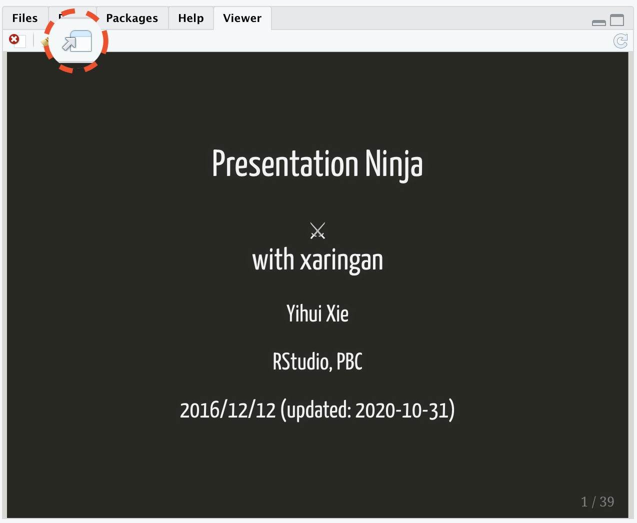
Addins \(\rightarrow\) Inifinite Moon Reader
xaringan slide \(\rightarrow\) browser
- We need to click
Inifinite Moon Readeronly to start the slideshow. To see the changes made in the slides just save the documentctrl + s