
Dr Ajay Kumar Koli
Head & Educator
School of Information & Data Science
Nalanda Academy - Wardha
@ajay_kolii
koliajaykumar@gmail.com
https://koliajay.netlify.app/
Hello! 😊
😍 R is FREE
- R is a language and environment for statistical computing and graphics. (R project)
😍 R is FREE
R is a language and environment for statistical computing and graphics. (R project)
In August 1993, designed by

Ross Ihaka
(New Zealand Statistician)

Robert Gentleman
(Canadian Statistician)

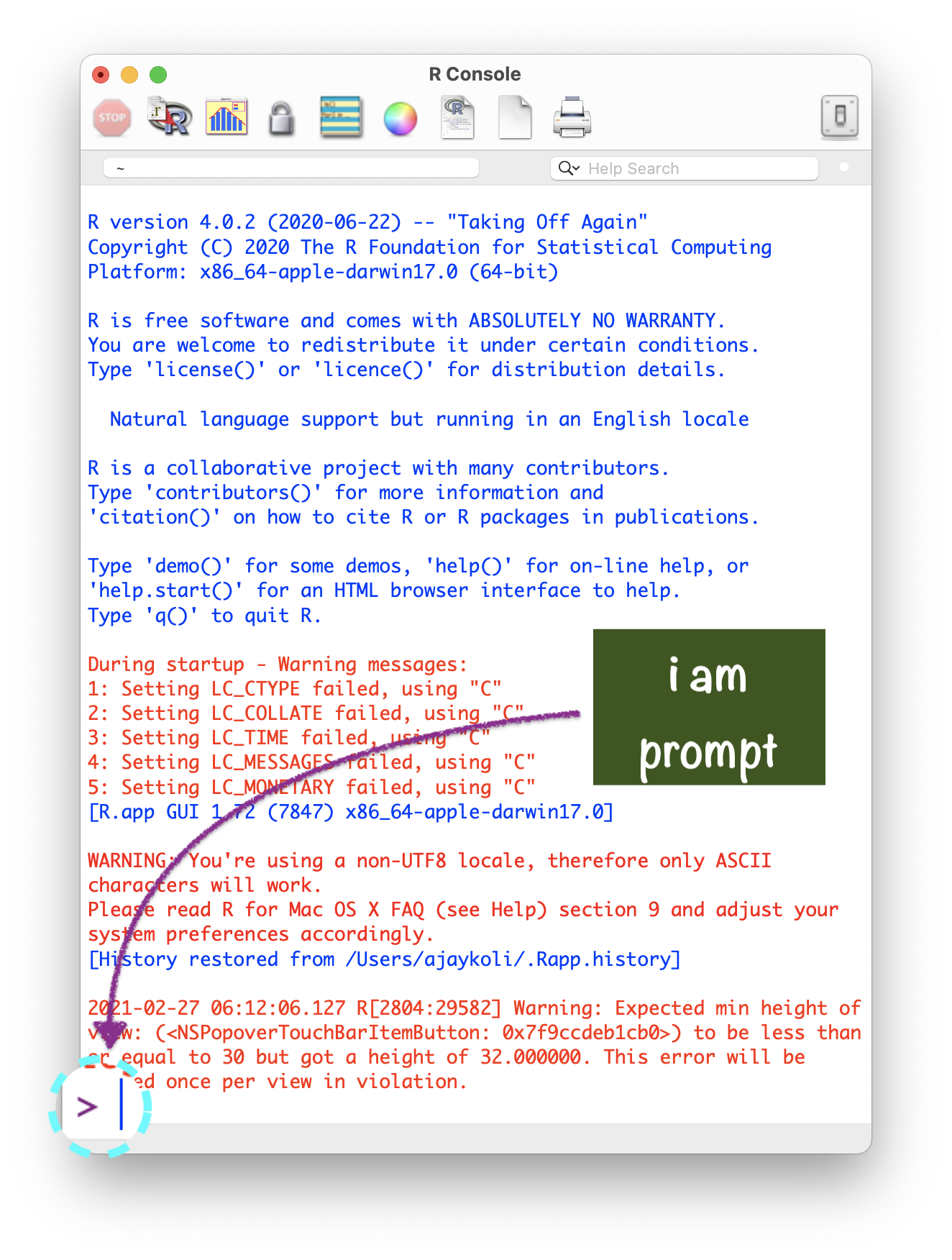
R Console
- R version
- R name
- R licence
- prompt >
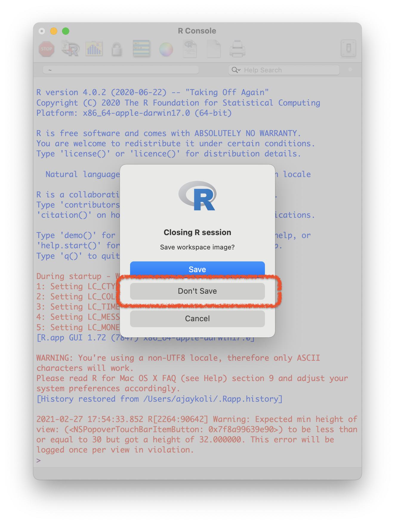
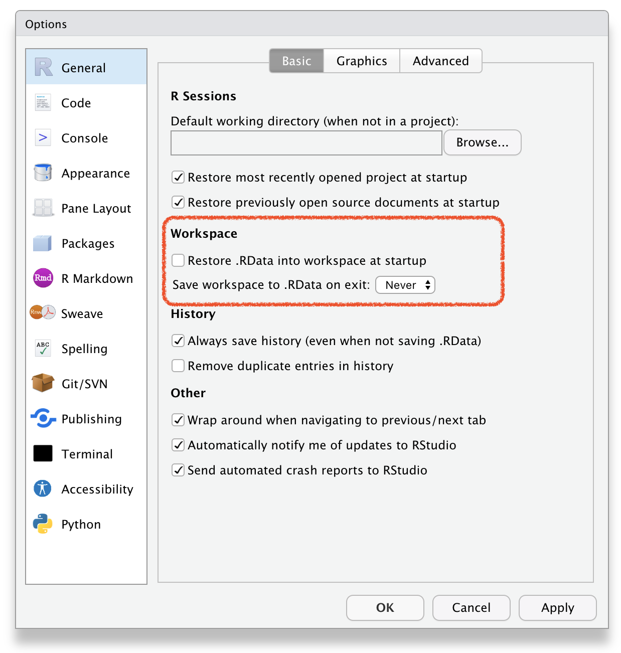
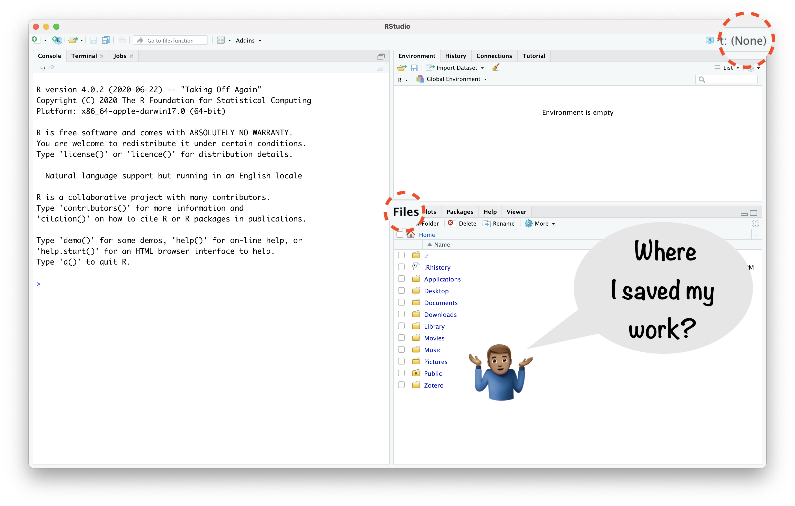
Never Save R "Workspace Image":
It helps in "freshly minted R sessions".
"put more trust in your script than in your memory"
R as a BIG calc
What you code
1What you see
## [1] 1R as a BIG calc
What you code
11 + 1What you see
## [1] 1## [1] 2R as a BIG calc
What you code
11 + 134 / 40What you see
## [1] 1## [1] 2## [1] 0.85R as a BIG calc
What you code
11 + 134 / 405 < 4What you see
## [1] 1## [1] 2## [1] 0.85## [1] FALSER as a BIG calc
What you code
11 + 134 / 405 < 416 == 16What you see
## [1] 1## [1] 2## [1] 0.85## [1] FALSE## [1] TRUE
Functions
R Function
- "A function, in a programming environment, is a set of instructions. A programmer builds a function to avoid repeating the same task, or reduce complexity."
Structure of R function
Comments
R Comment:
- "Humans will be able to read the comments, but your computer will pass over them."1
R Comment:
"Humans will be able to read the comments, but your computer will pass over them."1
In R,
#is used as a commenting symbol
😼 That's okay but you promise to...
😼 That's okay but you promise to...
- combine plot, text, tables and images in a single file.
😼 That's okay but you promise to...
combine plot, text, tables and images in a single file.
publish my work online or convert into a word, pdf or html file.
😼 That's okay but you promise to...
combine plot, text, tables and images in a single file.
publish my work online or convert into a word, pdf or html file.
work efficiently with my different projects and save, share and track them.
😼 That's okay but you promise to...
combine plot, text, tables and images in a single file.
publish my work online or convert into a word, pdf or html file.
work efficiently with my different projects and save, share and track them.
WE NEED A SUPERHERO ...
😻 About RStudio:
- 2009, Joseph J. Allaire founded RStudio.
😻 About RStudio:
2009, Joseph J. Allaire founded RStudio.
2011, RStudio IDE for R was launched.
😻 About RStudio:
2009, Joseph J. Allaire founded RStudio.
2011, RStudio IDE for R was launched.
"RStudio is dedicated to sustainable investment in free and open-source software for data science." (16 Jan 2022)
R ⇌ RStudio
R ⇌ RStudio
Imagine RStudio as a stylish car ...
🚗
R ⇌ RStudio
Imagine RStudio as a stylish car ...
🚗
and R as its powerful engine.
⚙️
RStudio IDE
RStudio → Tools → Global Options
RStudio → Tools → Global Options
R
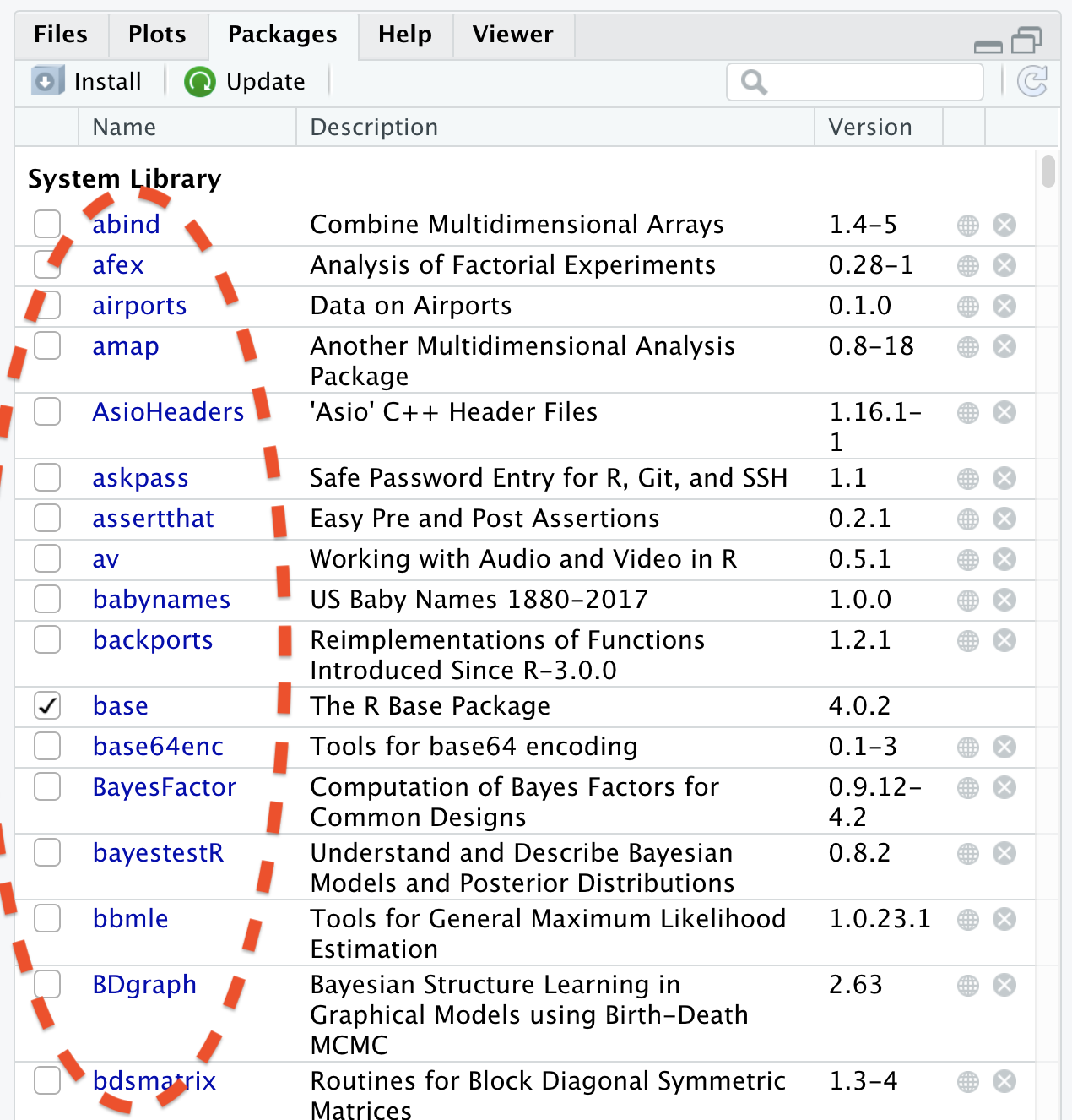
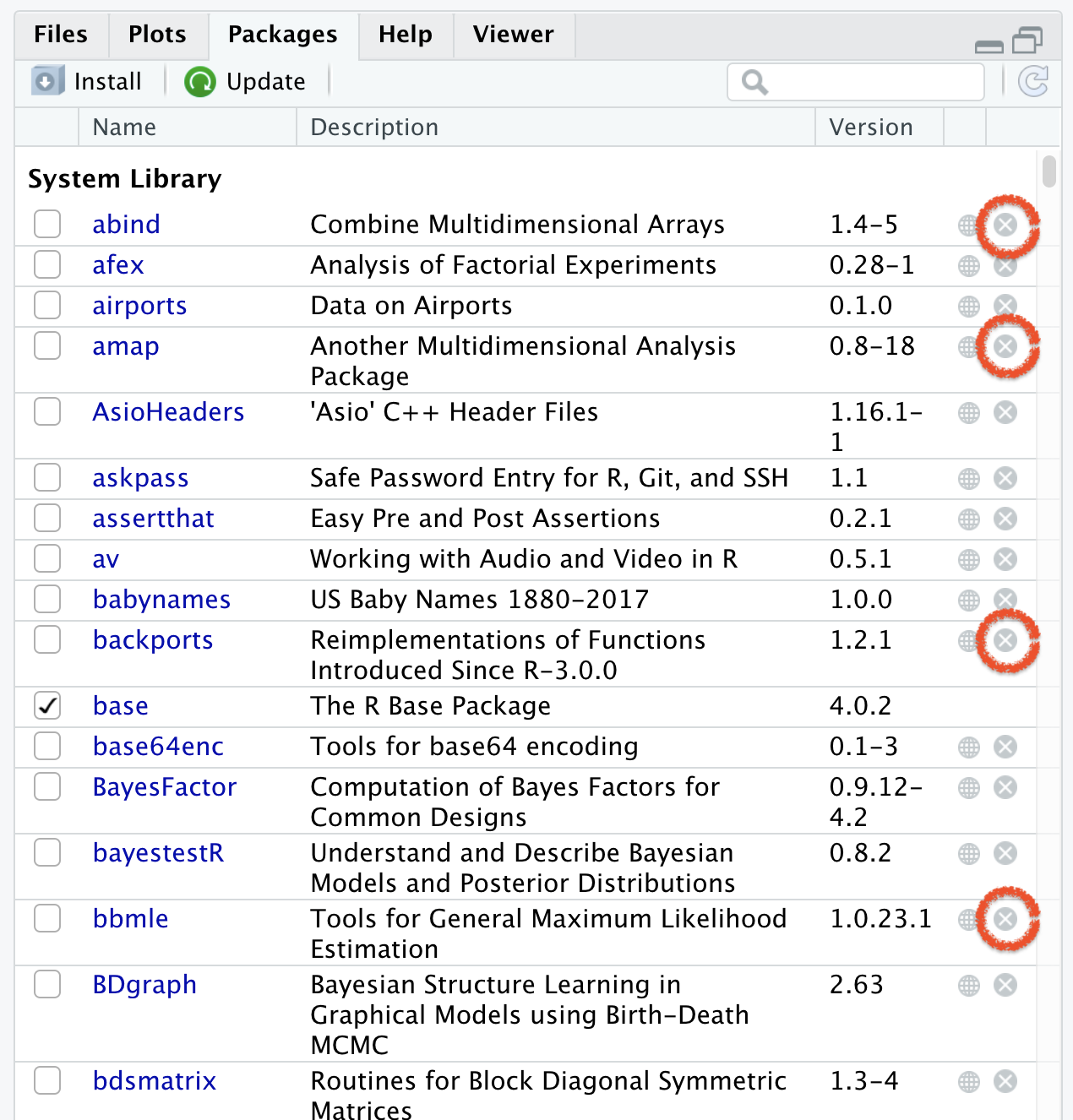
Packages
R Packages:
On 12 Jan 2022, 18698 R packages were available at CRAN
"An R package is a collection of functions, data, and documentation that extends the capabilities of base R. Using packages is key to the successful use of R."
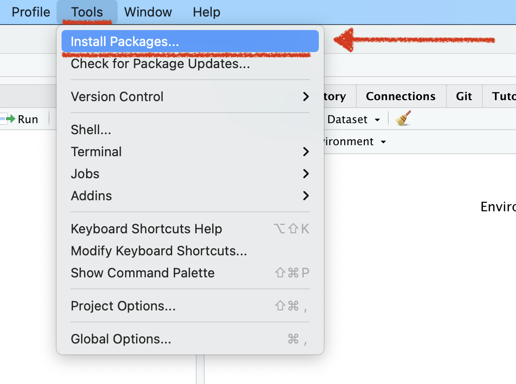
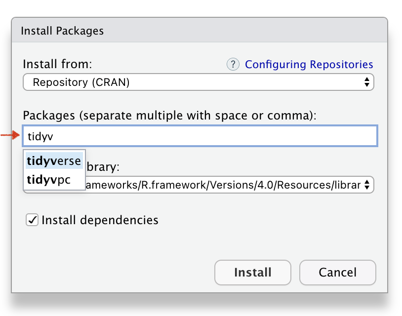
To Download pkgs
Name of the R package(s)
Installed R package(s)
R Function to Download Package
install.packages("tidyverse")R Function to Download Package
install.packages("tidyverse")R Function to use Package
library(tidyverse)About R Packages:
You need to install package only once like
- 📚 We buy books once and use them again and again
About R Packages:
You need to install package only once like
📚 We buy books once and use them again and again
💡 Fix the bulb once and use it again and again
About R Packages:
You need to install package only once like
📚 We buy books once and use them again and again
💡 Fix the bulb once and use it again and again
In every R document you need to
call oncethe package using functionlibrary(), for example library(ggplot2).
About R Packages:
You need to install package only once like
📚 We buy books once and use them again and again
💡 Fix the bulb once and use it again and again
In every R document you need to
call oncethe package using functionlibrary(), for example library(ggplot2).Once in a while, you need to update the installed packages as well.
- If you un-install R or RStudio, you will lose all installed packages.
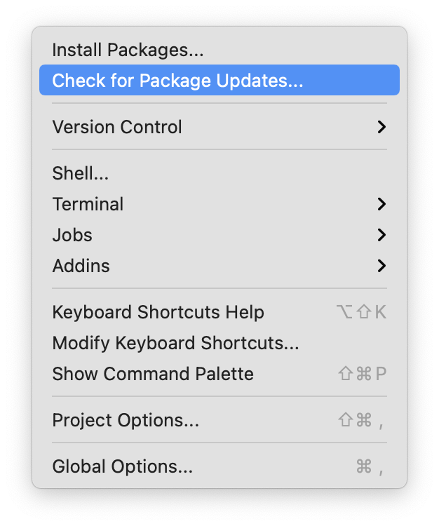
Tools → Check Package Updates
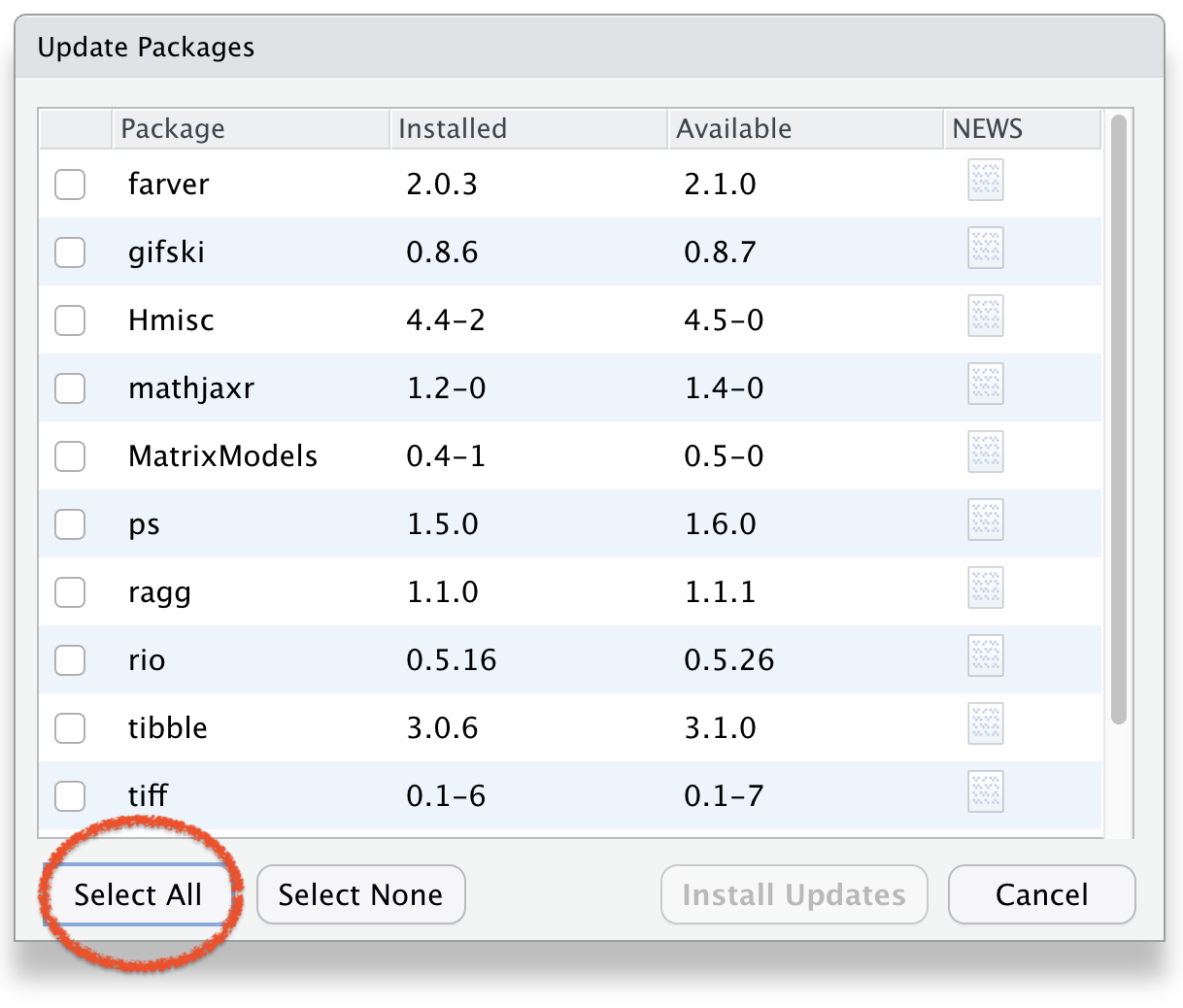
Select Package(s) to Update
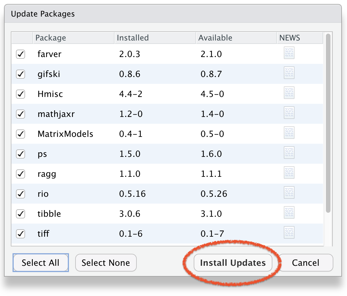
Click Install Updates
To Remove Package(s)
Objects
Guidelines to name objects in R:
- a name cannot start with a number
Guidelines to name objects in R:
a name cannot start with a number
a name cannot use some special symbols, like ^, !, $, @, +, -, /, or *:
Guidelines to name objects in R:
a name cannot start with a number
a name cannot use some special symbols, like ^, !, $, @, +, -, /, or *:
avoid caps
Guidelines to name objects in R:
a name cannot start with a number
a name cannot use some special symbols, like ^, !, $, @, +, -, /, or *:
avoid caps
avoid space
Guidelines to name objects in R:
a name cannot start with a number
a name cannot use some special symbols, like ^, !, $, @, +, -, /, or *:
avoid caps
avoid space
- use dash (like na-me) or underscore (like na_me)
Guidelines to name objects in R:
a name cannot start with a number
a name cannot use some special symbols, like ^, !, $, @, +, -, /, or *:
avoid caps
avoid space
use dash (like na-me) or underscore (like na_me)
if chronology matters then add date (2020-09-05-file-name)
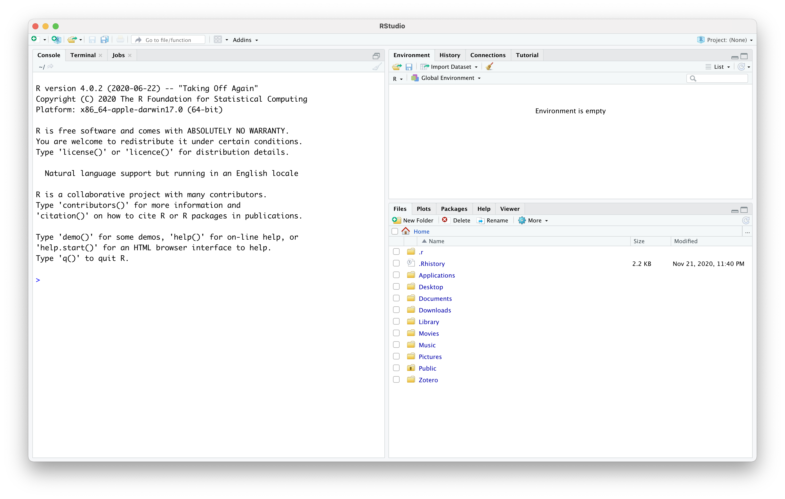
RStudio Environment Window
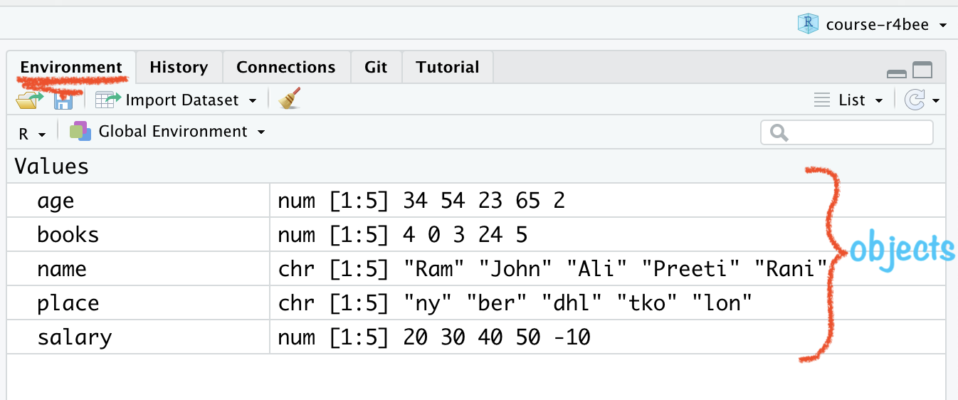
RStudio Environment Window
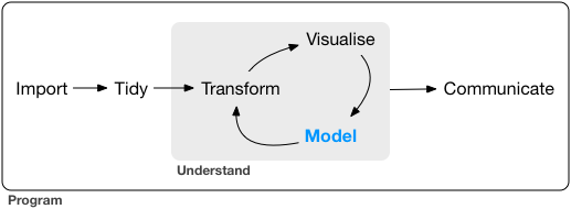
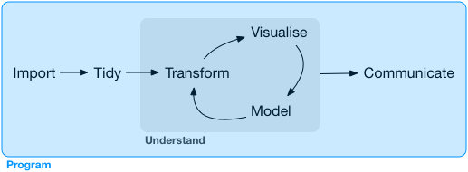
🤔how to combine these
objects/variables into a data or say tidy data
Tidy data 👇 😻😻😻
## age books name place salary## 1 34 4 Ram ny 20## 2 54 0 Rani ber 30## 3 23 3 Ali dhl 40## 4 65 24 Preeti tko 50## 5 2 5 John lon -10Tidy data 👇 😻😻😻
## age books name place salary## 1 34 4 Ram ny 20## 2 54 0 Rani ber 30## 3 23 3 Ali dhl 40## 4 65 24 Preeti tko 50## 5 2 5 John lon -10
🧠 YOUR TURN
Write codes for below dataframe
## state pop capital foundation## 1 Germany 20 Berlin 1870-12-10## 2 France 19 Paris 1789-07-14## 3 India 50 Delhi 1947-08-15## 4 Russia 25 Moscow 1990-06-12## 5 USA 30 Washington 1776-07-04## 6 New Zealand 5 Wellington 1840-02-06state <- c("Germany", "France", "India", "Russia", "USA", "New Zealand")pop <- c(20, 19, 50, 25, 30, 5)capital <- c("Berlin", "Paris", "Delhi", "Moscow", "Washington", "Wellington")foundation <- c("1870-12-10", "1789-07-14", "1947-08-15", "1990-06-12", "1776-07-04", "1840-02-06")world <- data.frame(state, pop, capital, foundation)world10:00
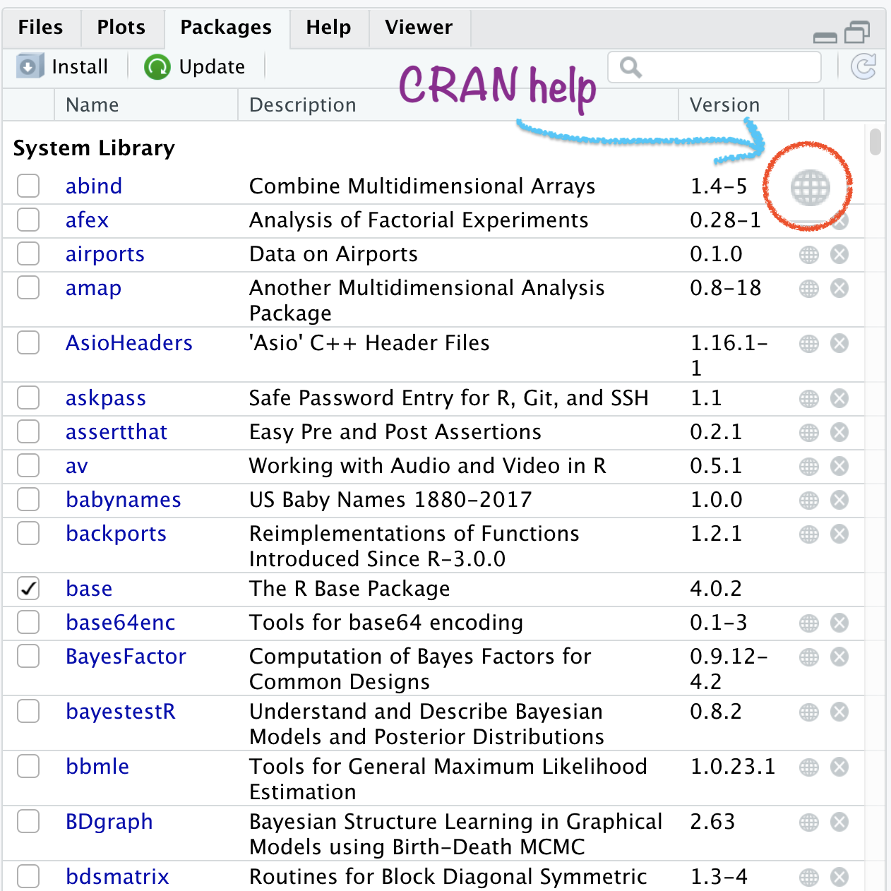
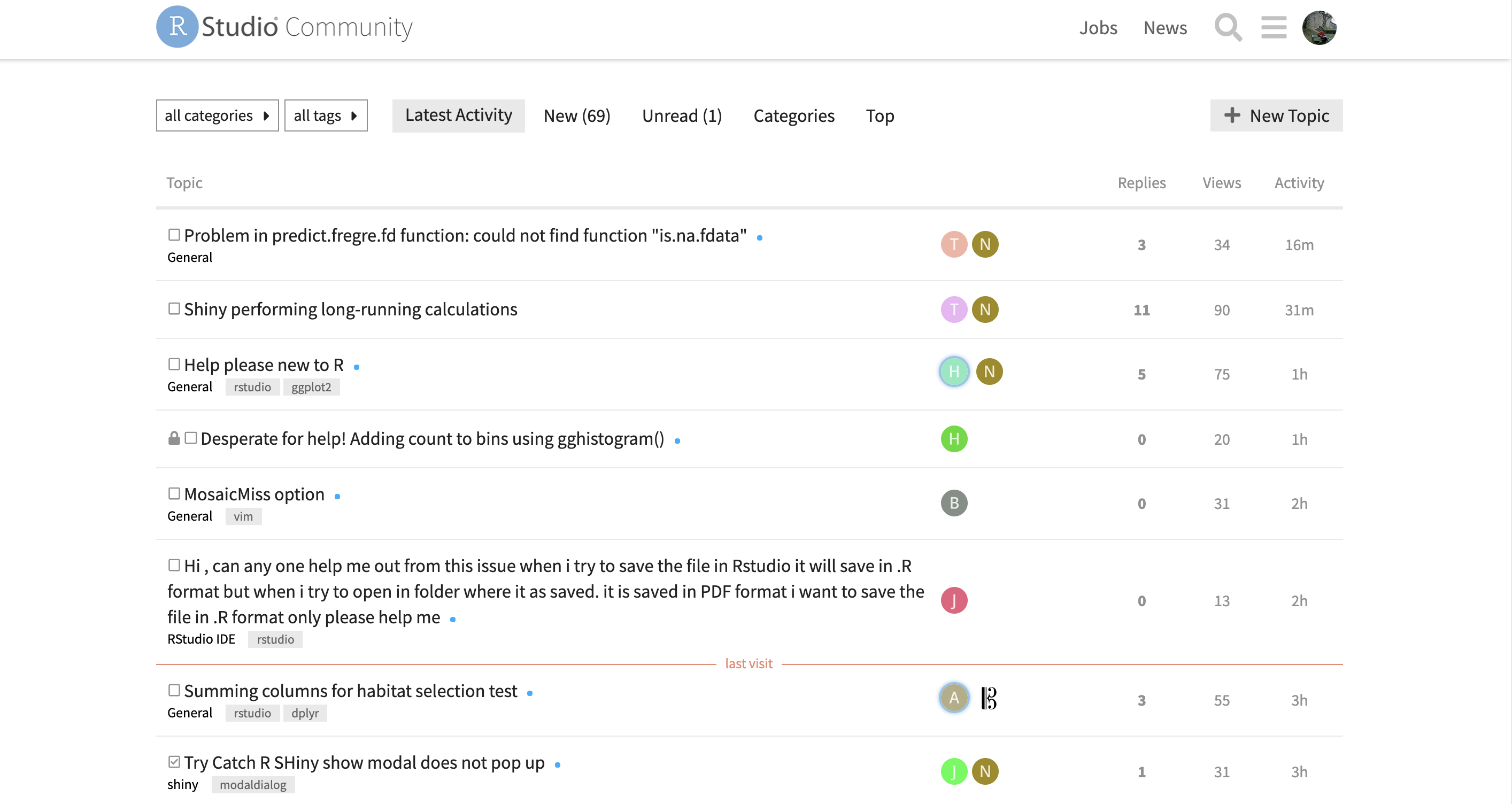
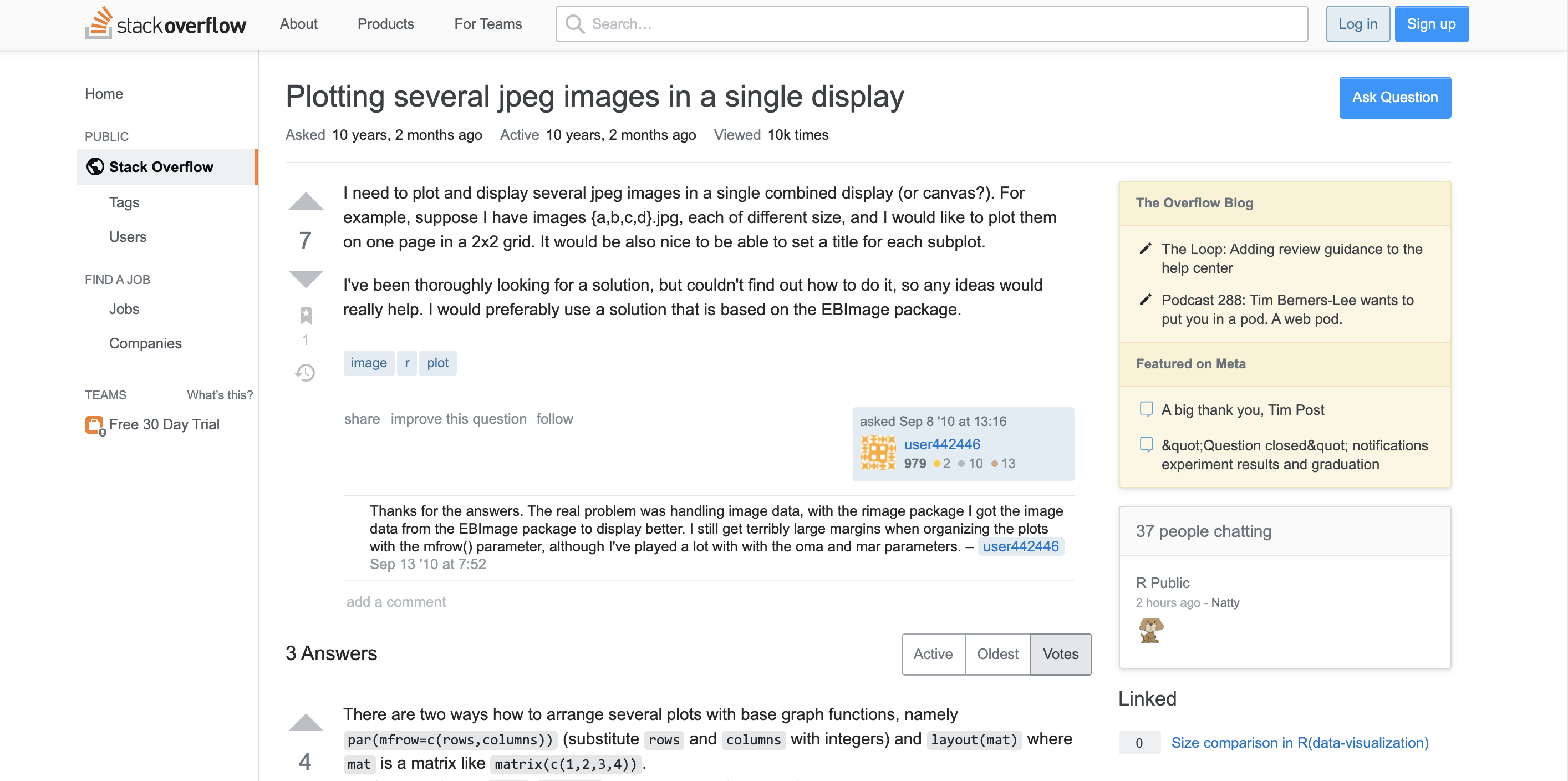
Need Help!
Using Console >
in console type ?your query
Using Console >
in console type ?your query
for example ?ggplot
RStudio: pkg Help Docs
🙋🏽♀️🙋♂️
Q&A
Dynamic Documents
Using R Markdown
Next Module - 2
Open RStudio
Open RStudio
Open RStudio
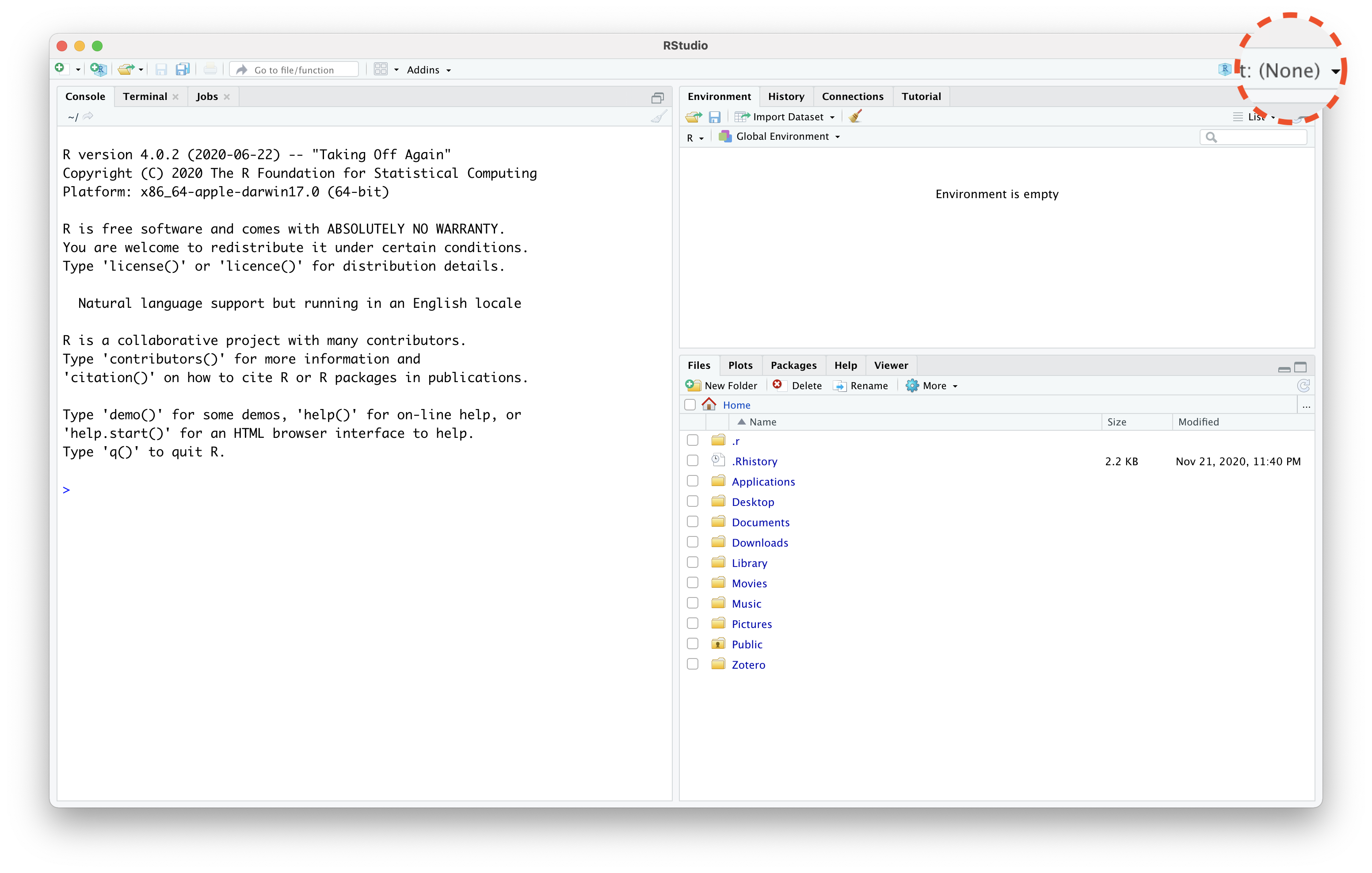
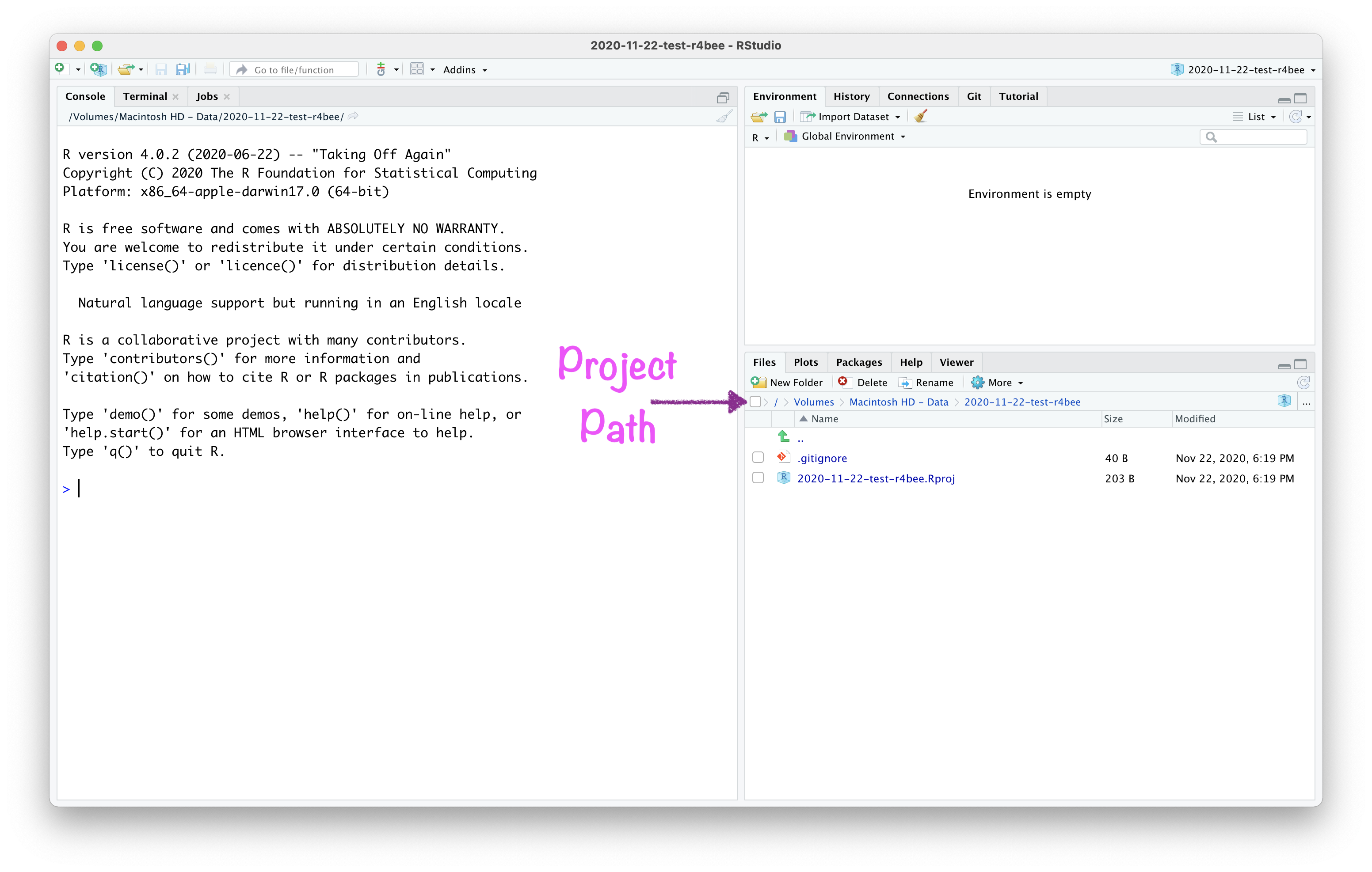
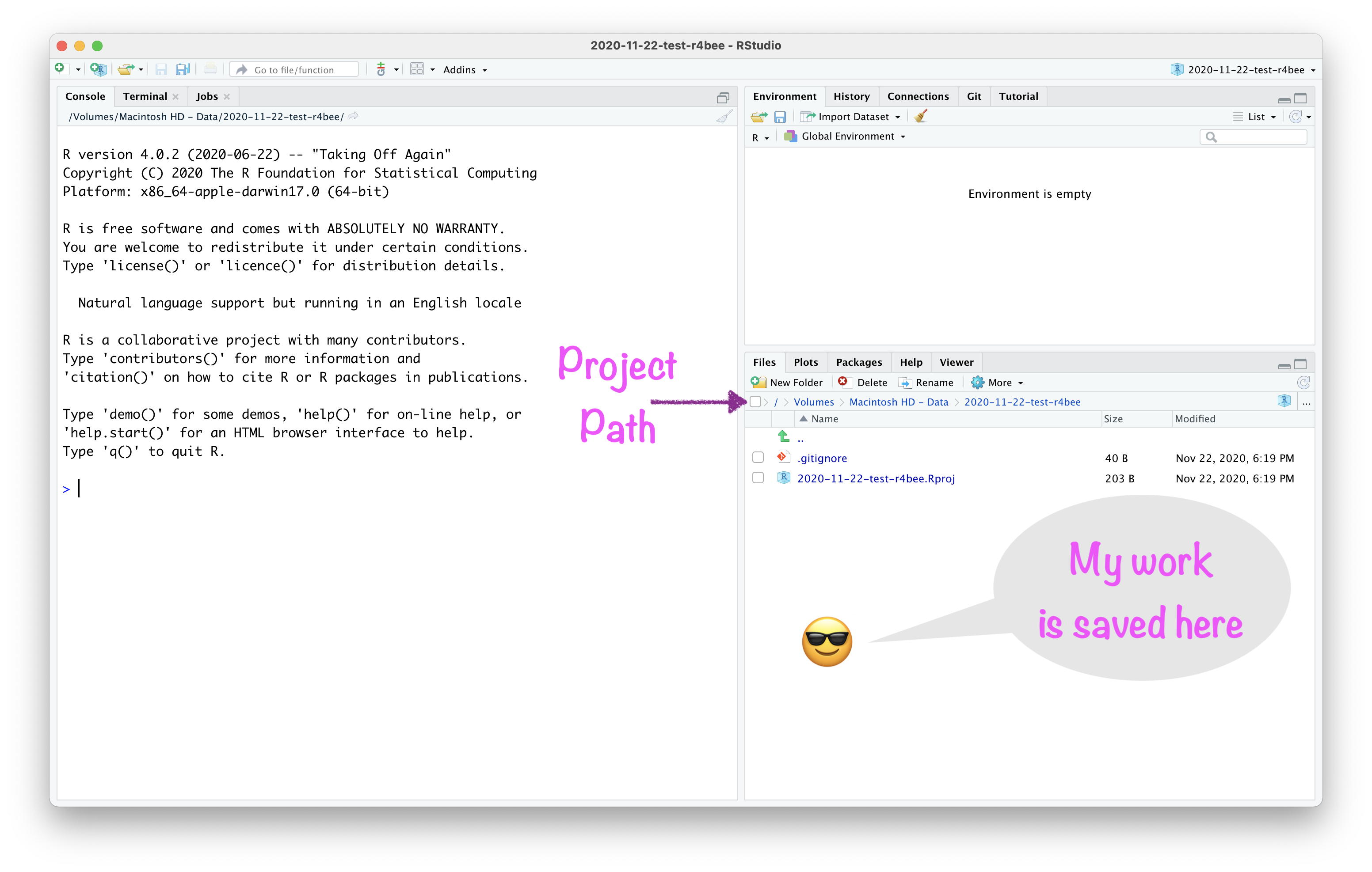
RStudio
Project
About RStudio Projects
- "to divide your work into multiple contexts, each with their own:
About RStudio Projects
"to divide your work into multiple contexts, each with their own:
- working directory,
About RStudio Projects
"to divide your work into multiple contexts, each with their own:
working directory,
workspace,
About RStudio Projects
"to divide your work into multiple contexts, each with their own:
working directory,
workspace,
history, and
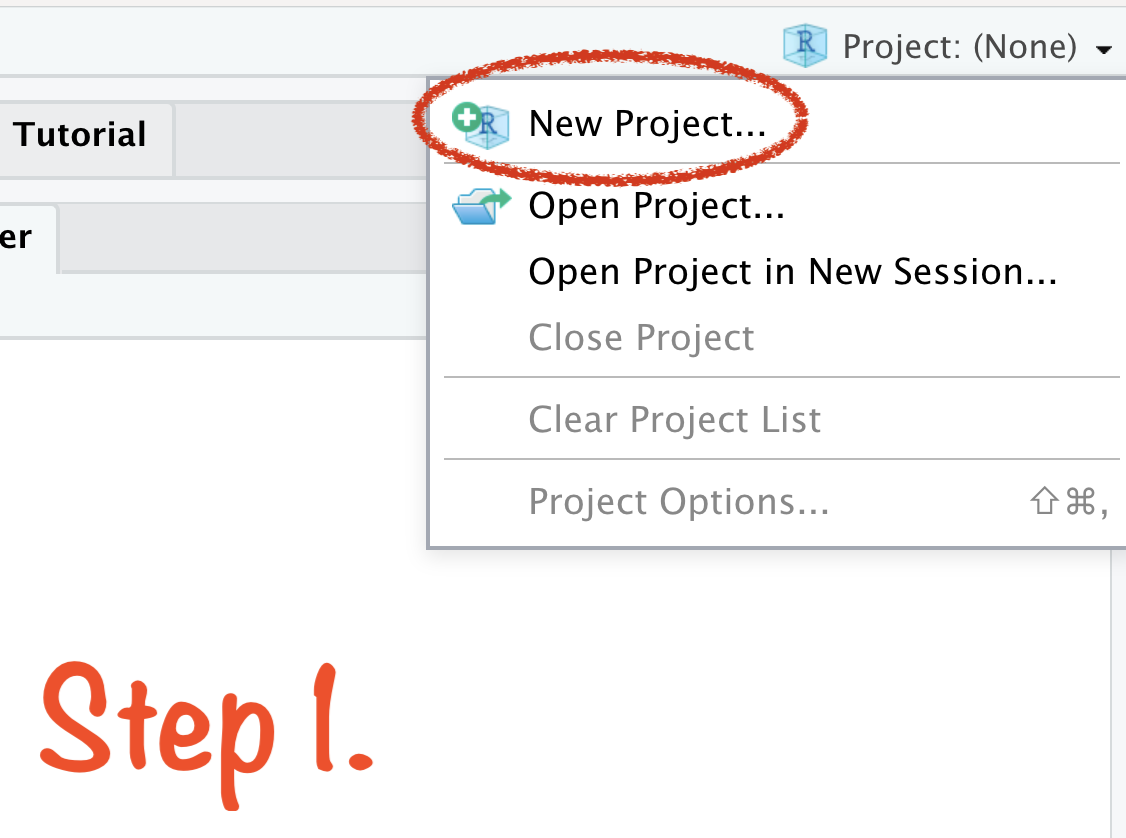
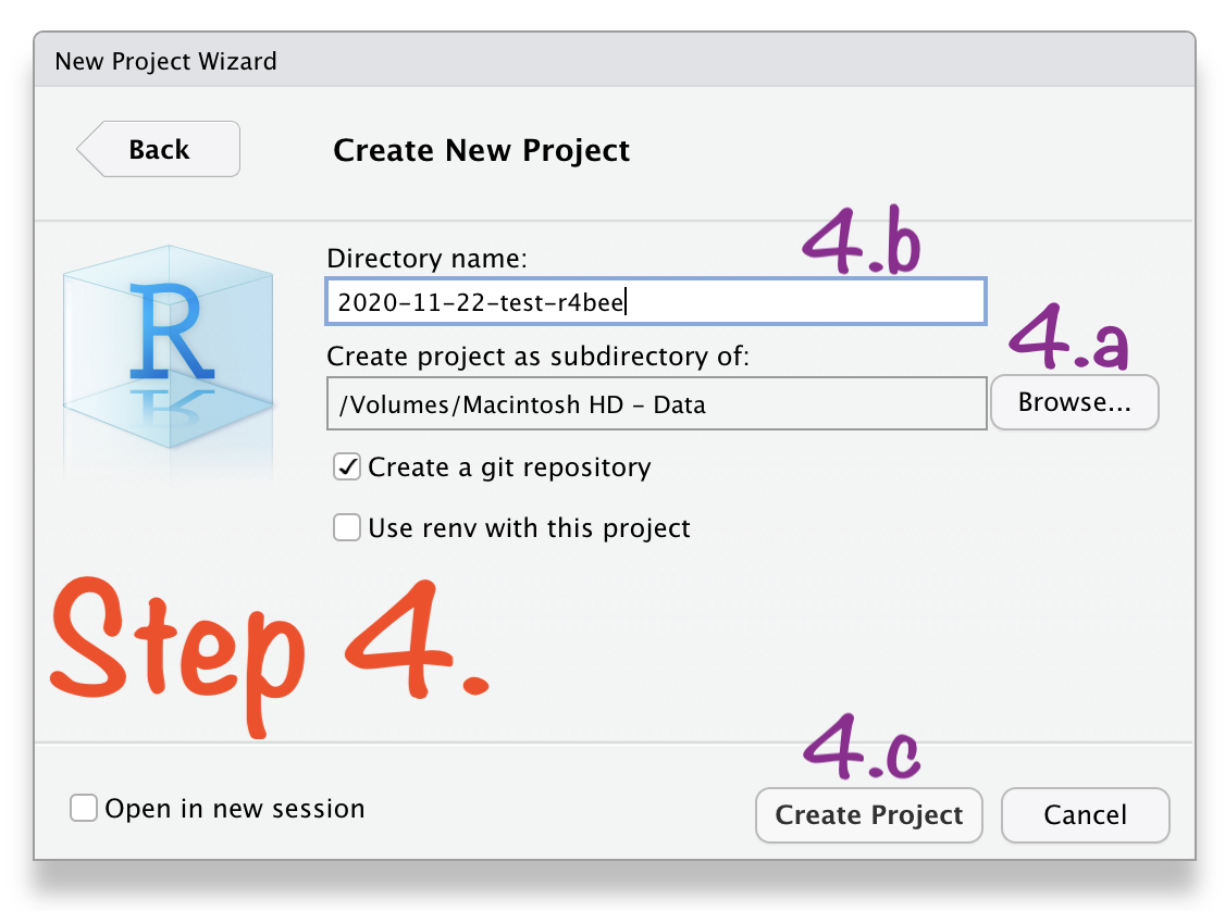
🔥 Create RStudio Project in 4 Steps 🔥
Create RStudio Project in 4 Steps
Create RStudio Project in 4 Steps
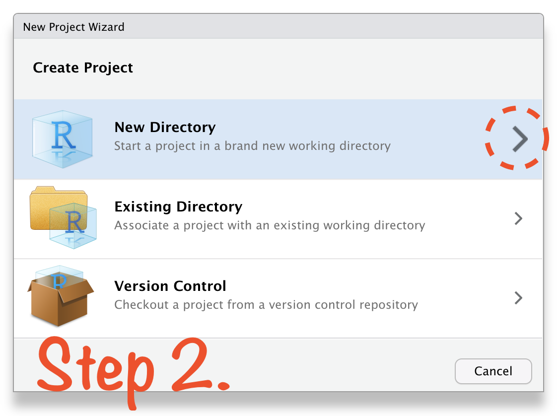
Create RStudio Project in 4 Steps
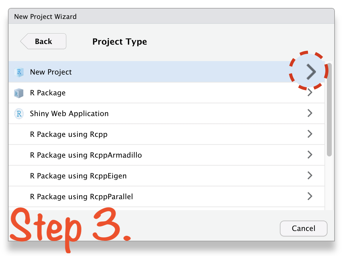
Create RStudio Project in 4 Steps
Open RStudio Project
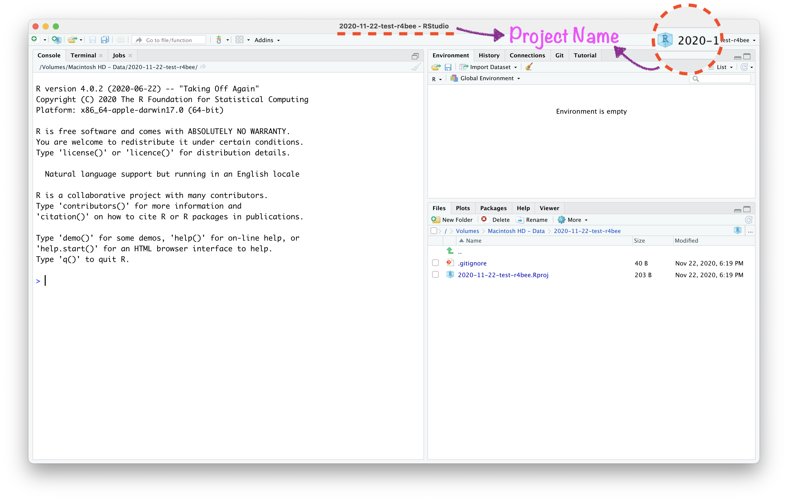
Open RStudio Project
Open RStudio Project
R
Package
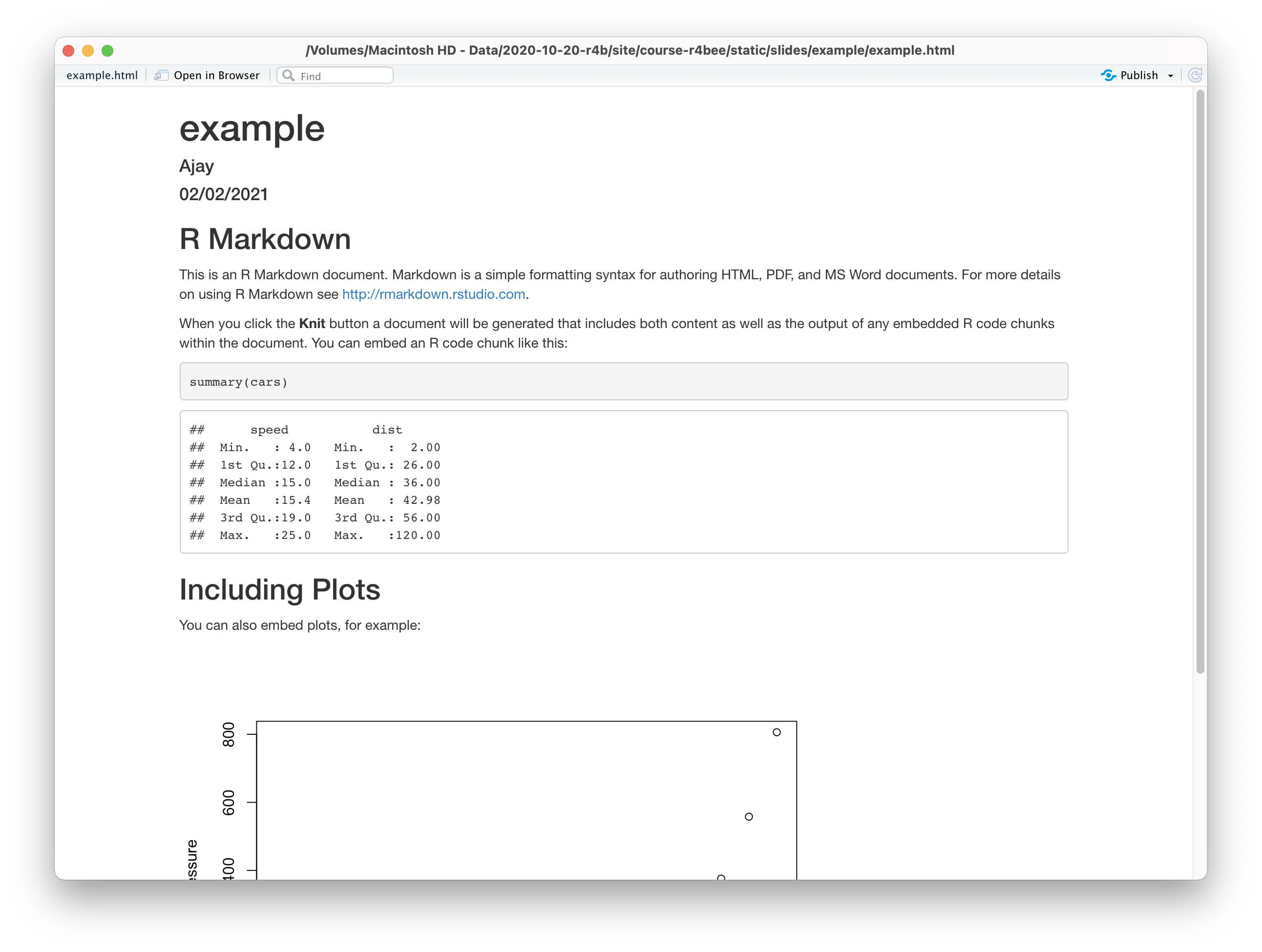
About R Markdown:
- "You bring your data, code, and ideas, and R Markdown renders your content into a polished document that can be used to:
About R Markdown:
"You bring your data, code, and ideas, and R Markdown renders your content into a polished document that can be used to:
- Do data science interactively within the RStudio IDE,
About R Markdown:
"You bring your data, code, and ideas, and R Markdown renders your content into a polished document that can be used to:
Do data science interactively within the RStudio IDE,
Reproduce your analyses,
About R Markdown:
"You bring your data, code, and ideas, and R Markdown renders your content into a polished document that can be used to:
Do data science interactively within the RStudio IDE,
Reproduce your analyses,
Collaborate and share code with others, and
About R Markdown:
"You bring your data, code, and ideas, and R Markdown renders your content into a polished document that can be used to:
Do data science interactively within the RStudio IDE,
Reproduce your analyses,
Collaborate and share code with others, and
Communicate your results with others."
What is R Markdown? from RStudio, Inc. on Vimeo.
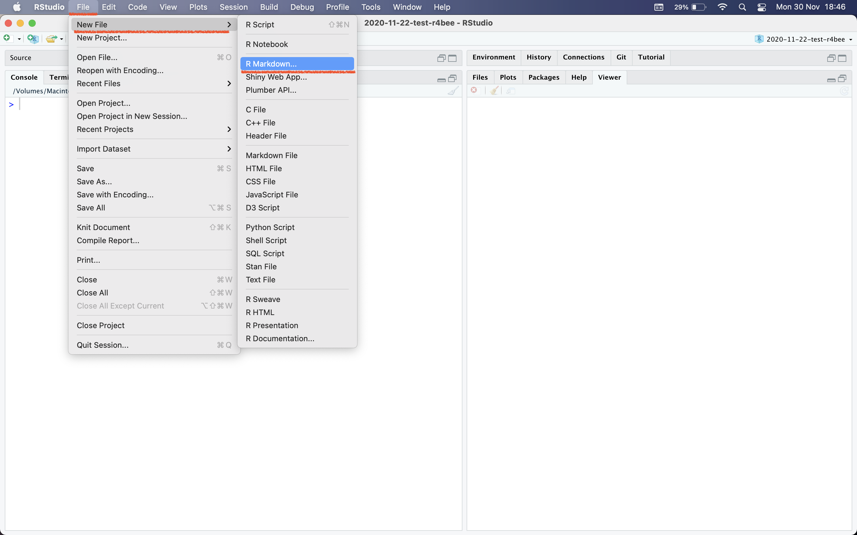
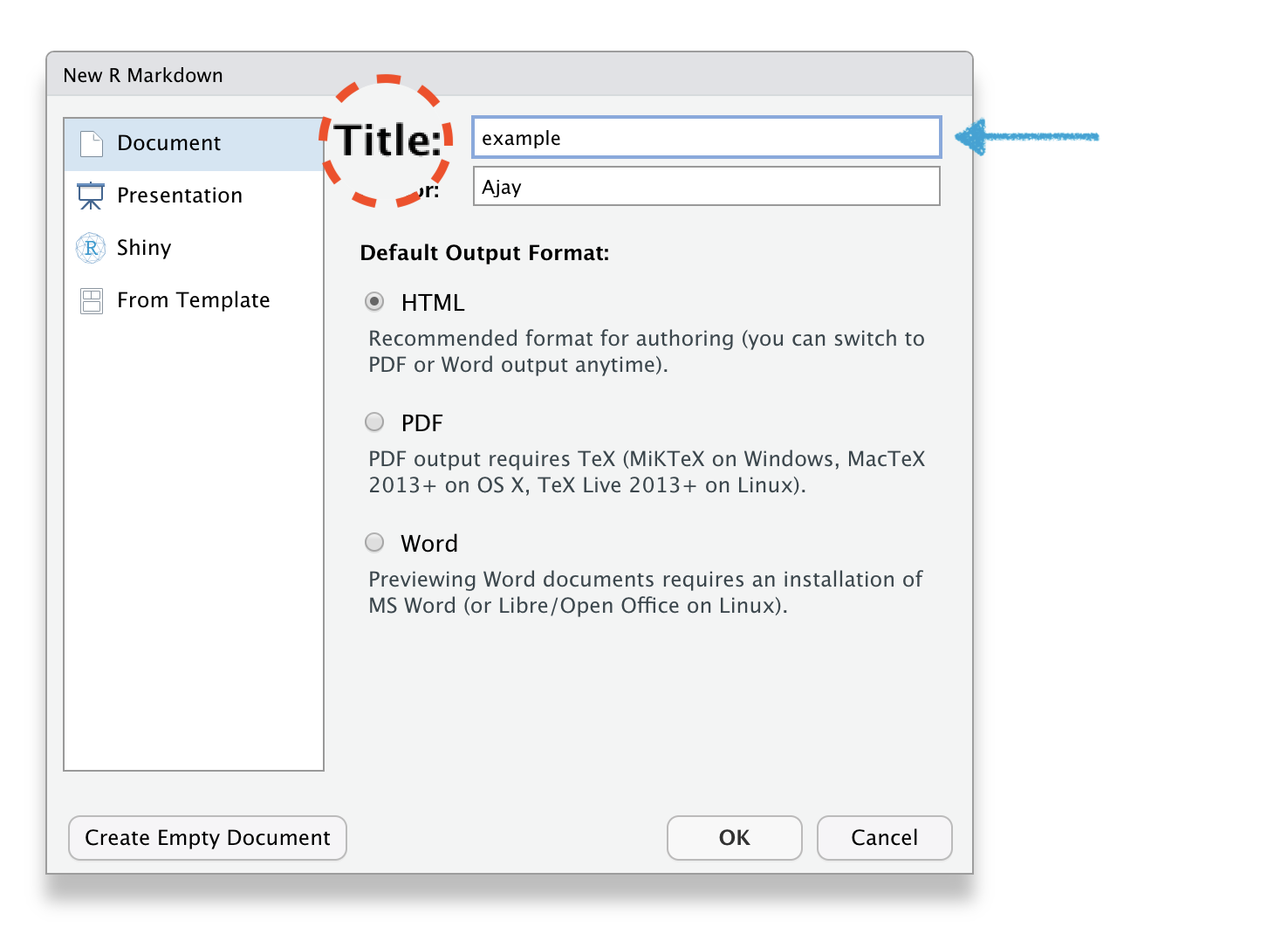
🔥How to create R Markdown file?🔥
File → New File → R Markdown
R Markdown
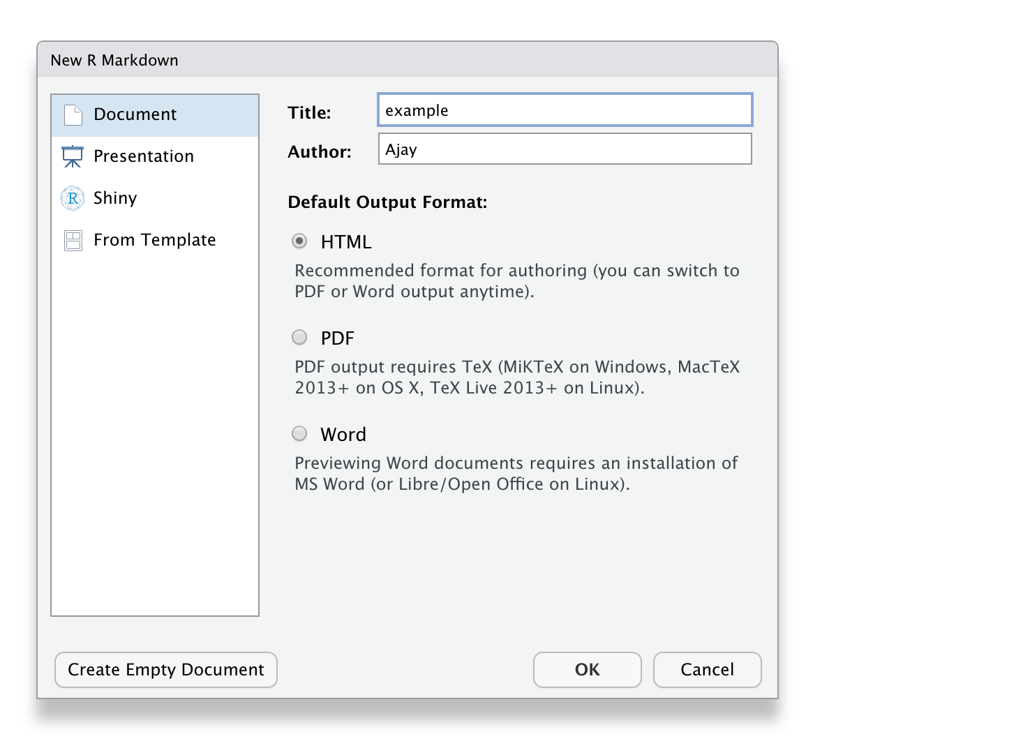
R Markdown
R Markdown
R Markdown

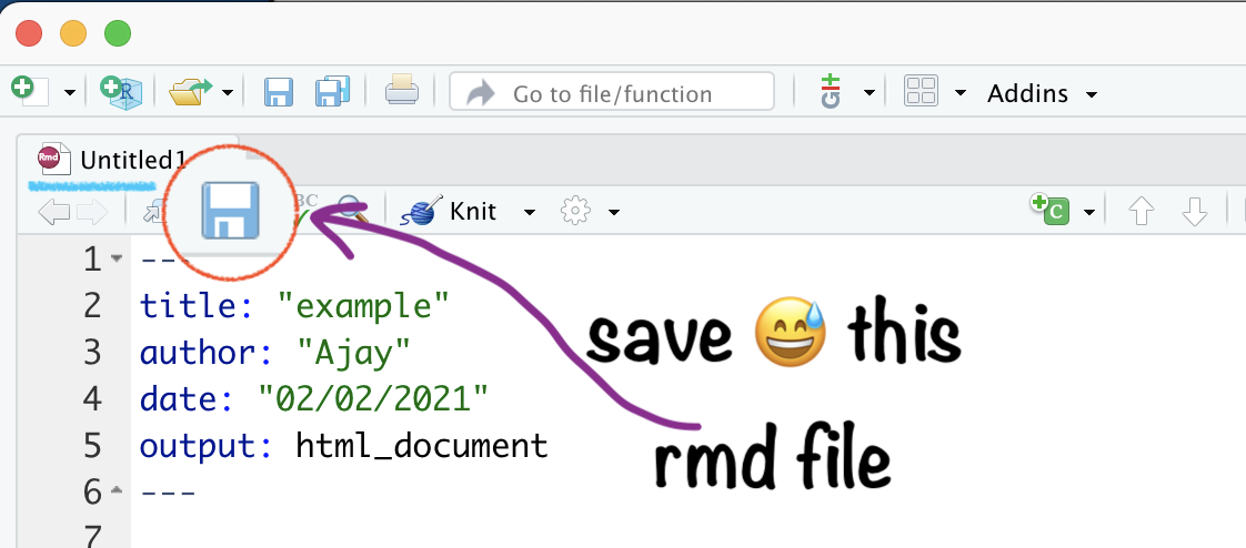
Save your .Rmd file
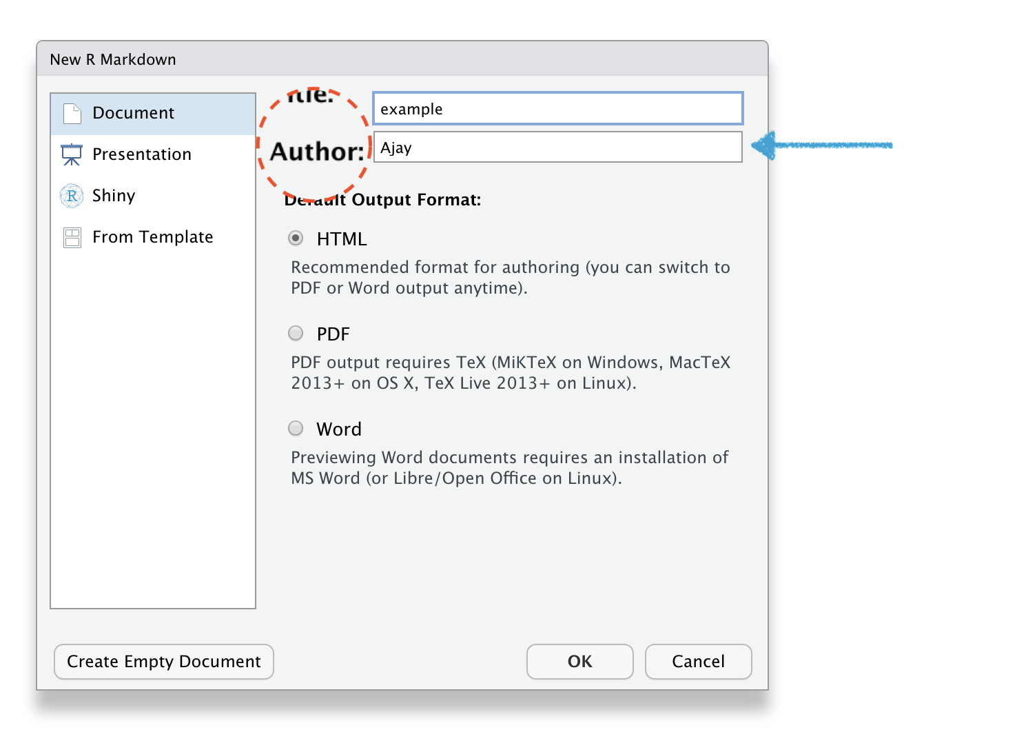
Name your .Rmd file
Name your .Rmd file
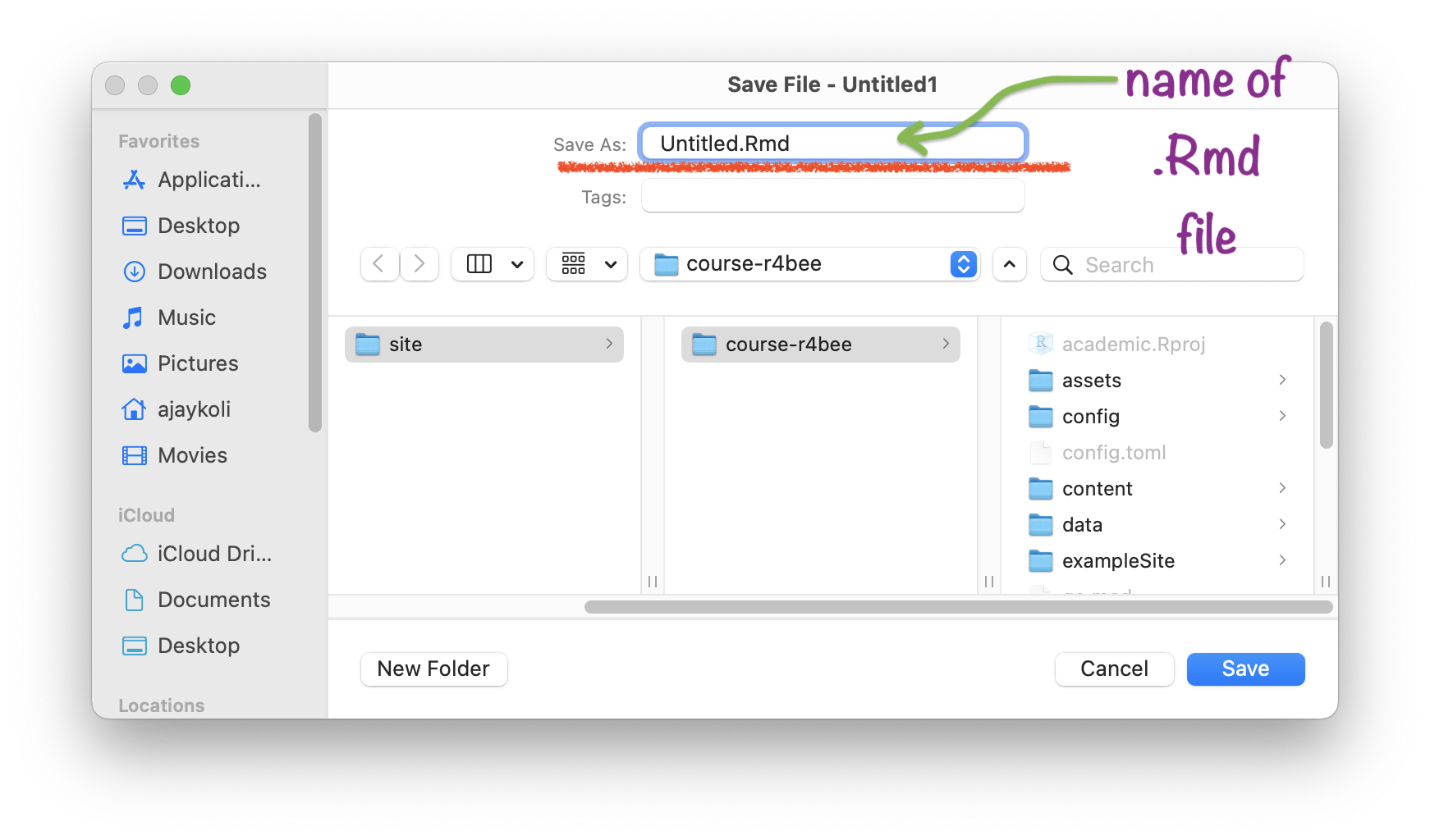
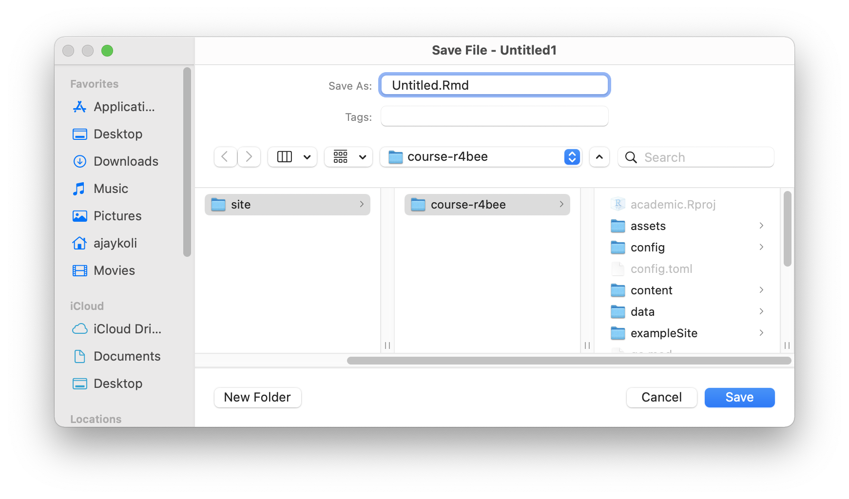
Save your .Rmd file
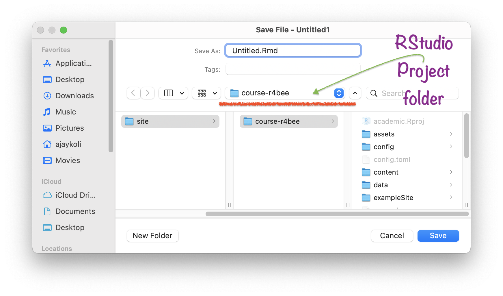
Saved .Rmd file → in RStudio Project
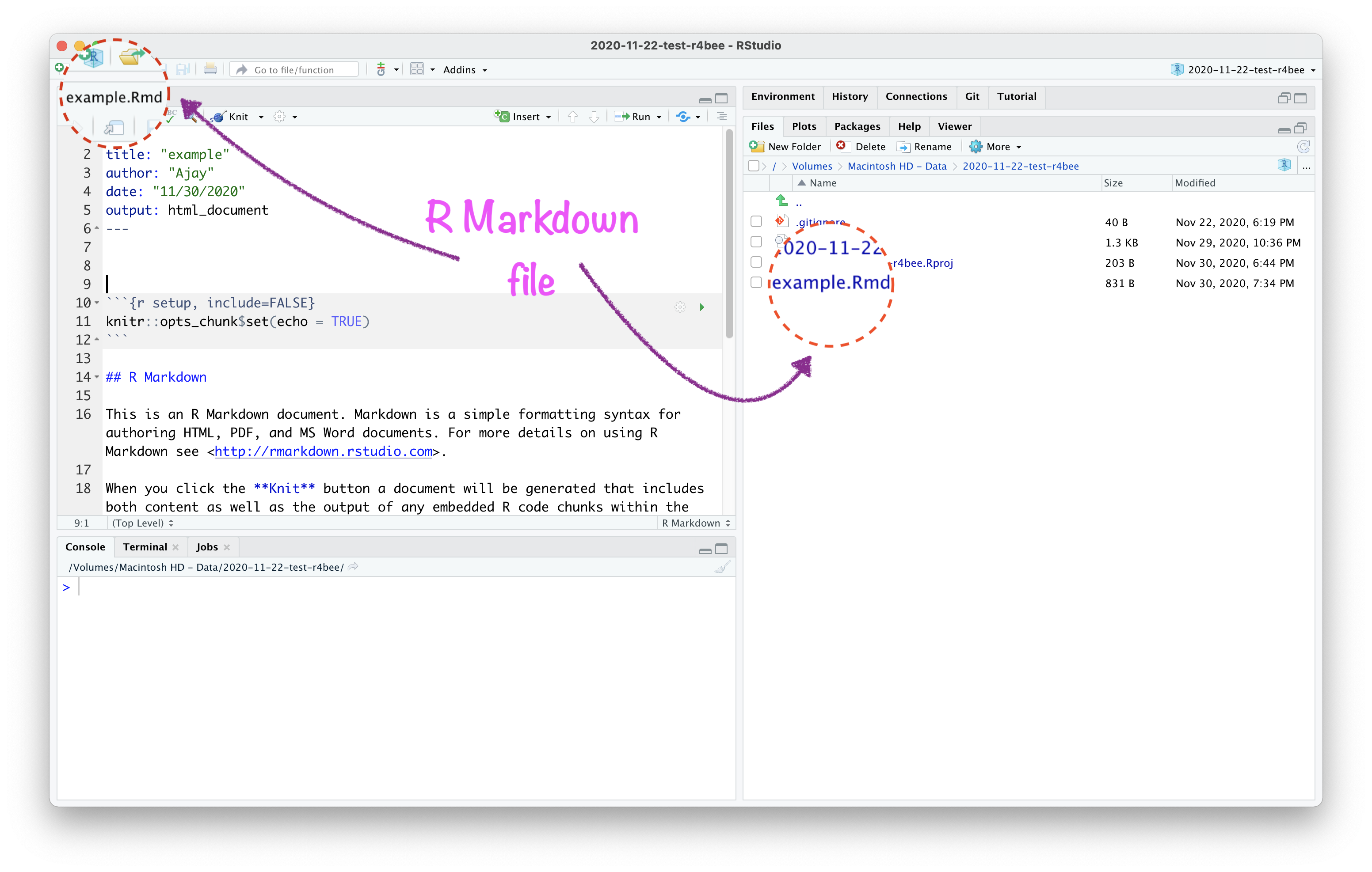
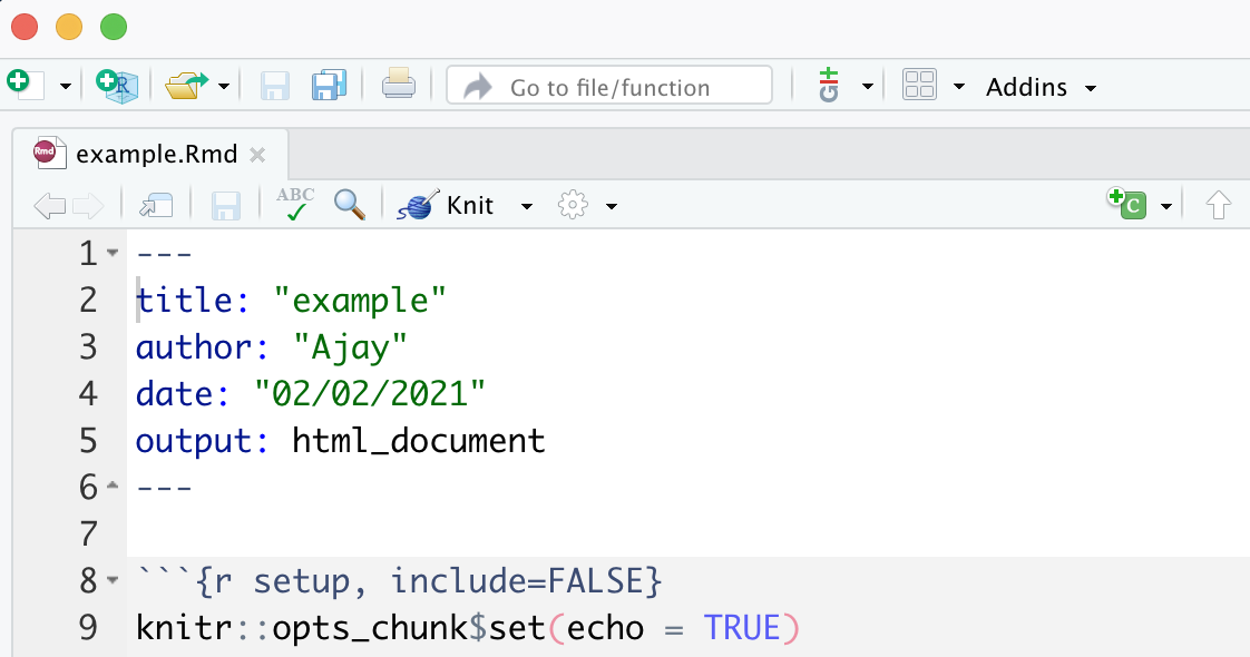
R Markdown has 3 important parts:
- YAML
- Code chunk
- Text
🧶 Knit a R Markdown File
YAML options
Headings, subheadings, text & maths equations
Code Chunk
Include images
Include tables
Include plot
Themes
Multiple Output Formats
🙋🏽♀️🙋♂️
Q&A
Dynamic Visualisation
Using ggplot2
Next Module - 3
Course Progress
Variable types in R:
Variable types in R:
intstands for integers, like 4, 55, 300.
Variable types in R:
intstands for integers, like 4, 55, 300.dblstands for doubles, or real numbers like 3, 7.45, 1.565, 12.
Variable types in R:
intstands for integers, like 4, 55, 300.dblstands for doubles, or real numbers like 3, 7.45, 1.565, 12.chrstands for character vectors, or strings like names.
Variable types in R:
intstands for integers, like 4, 55, 300.dblstands for doubles, or real numbers like 3, 7.45, 1.565, 12.chrstands for character vectors, or strings like names.dttmstands for date-times (a date + a time).
Variable types in R:
intstands for integers, like 4, 55, 300.dblstands for doubles, or real numbers like 3, 7.45, 1.565, 12.chrstands for character vectors, or strings like names.dttmstands for date-times (a date + a time).lglstands for logical, vectors that contain only TRUE or FALSE.
Variable types in R:
intstands for integers, like 4, 55, 300.dblstands for doubles, or real numbers like 3, 7.45, 1.565, 12.chrstands for character vectors, or strings like names.dttmstands for date-times (a date + a time).lglstands for logical, vectors that contain only TRUE or FALSE.fctstands for factors, which R uses to represent categorical variables with fixed possible values like occupation: student, professional, government, business.
Variable types in R:
intstands for integers, like 4, 55, 300.dblstands for doubles, or real numbers like 3, 7.45, 1.565, 12.chrstands for character vectors, or strings like names.dttmstands for date-times (a date + a time).lglstands for logical, vectors that contain only TRUE or FALSE.fctstands for factors, which R uses to represent categorical variables with fixed possible values like occupation: student, professional, government, business.datestands for dates.
Data of Palmer Penguins
- It comes with R package
palmerpenguins
Data of Palmer Penguins
It comes with R package
palmerpenguinsName of the data is
penguins
Data of Palmer Penguins
It comes with R package
palmerpenguinsName of the data is
penguinsTo know more about the data
?penguins
Data of Palmer Penguins
It comes with R package
palmerpenguinsName of the data is
penguinsTo know more about the data
?penguinsIncluded variables are:
- species, island, bill_length_mm, bill_depth_mm, flipper_length_mm, body_mass_g, sex, year
An Overview of Data
glimpse(penguins)## Rows: 344## Columns: 8## $ species <fct> Adelie, Adelie, …## $ island <fct> Torgersen, Torge…## $ bill_length_mm <dbl> 39.1, 39.5, 40.3…## $ bill_depth_mm <dbl> 18.7, 17.4, 18.0…## $ flipper_length_mm <int> 181, 186, 195, N…## $ body_mass_g <int> 3750, 3800, 3250…## $ sex <fct> male, female, fe…## $ year <int> 2007, 2007, 2007…An Overview of Data
summary(penguins)## species island ## Adelie :152 Biscoe :168 ## Chinstrap: 68 Dream :124 ## Gentoo :124 Torgersen: 52 ## ## ## ## ## bill_length_mm bill_depth_mm ## Min. :32.10 Min. :13.10 ## 1st Qu.:39.23 1st Qu.:15.60 ## Median :44.45 Median :17.30 ## Mean :43.92 Mean :17.15 ## 3rd Qu.:48.50 3rd Qu.:18.70 ## Max. :59.60 Max. :21.50 ## NA's :2 NA's :2 ## flipper_length_mm body_mass_g ## Min. :172.0 Min. :2700 ## 1st Qu.:190.0 1st Qu.:3550 ## Median :197.0 Median :4050 ## Mean :200.9 Mean :4202 ## 3rd Qu.:213.0 3rd Qu.:4750 ## Max. :231.0 Max. :6300 ## NA's :2 NA's :2 ## sex year ## female:165 Min. :2007 ## male :168 1st Qu.:2007 ## NA's : 11 Median :2008 ## Mean :2008 ## 3rd Qu.:2009 ## Max. :2009 ##Packages required:
library(palmerpenguins) # to access penguin datalibrary(tidyverse) # to use ggplot2 pkg- Packages recommended:
install.packages(c( "directlabels", "dplyr", "gameofthrones", "ggforce", "gghighlight", "ggnewscale", "ggplot2", "ggraph", "ggrepel", "ggtext", "ggthemes", "hexbin", "mapproj", "maps", "munsell", "ozmaps", "paletteer", "patchwork", "rmapshaper", "scico", "seriation", "sf", "stars", "tidygraph", "tidyr", "wesanderson" ))R
Package
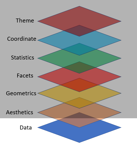
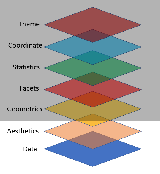
ggplot2 by Hadley Wickham
- "is a system for declaratively creating graphics, based on The Grammar of Graphics" (book by Late Leland Wilkinson)

Late Leland Wilkinson
Hadley Wickham
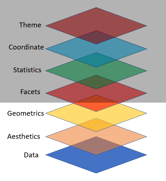
Key Components for ggplot2 Plot
data,
aesthetic mapping
at least one layer of geom function


How to export plot to your computer?

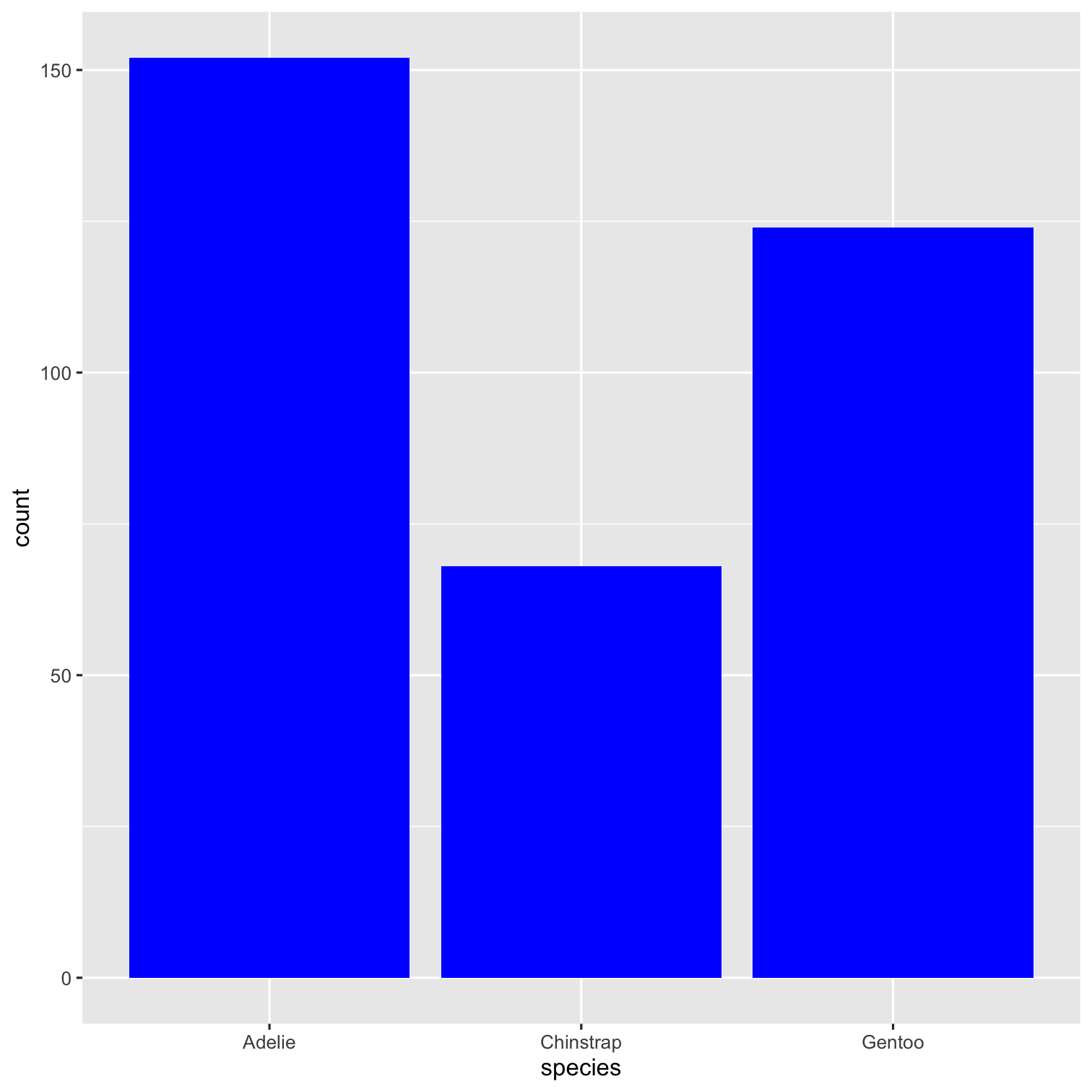
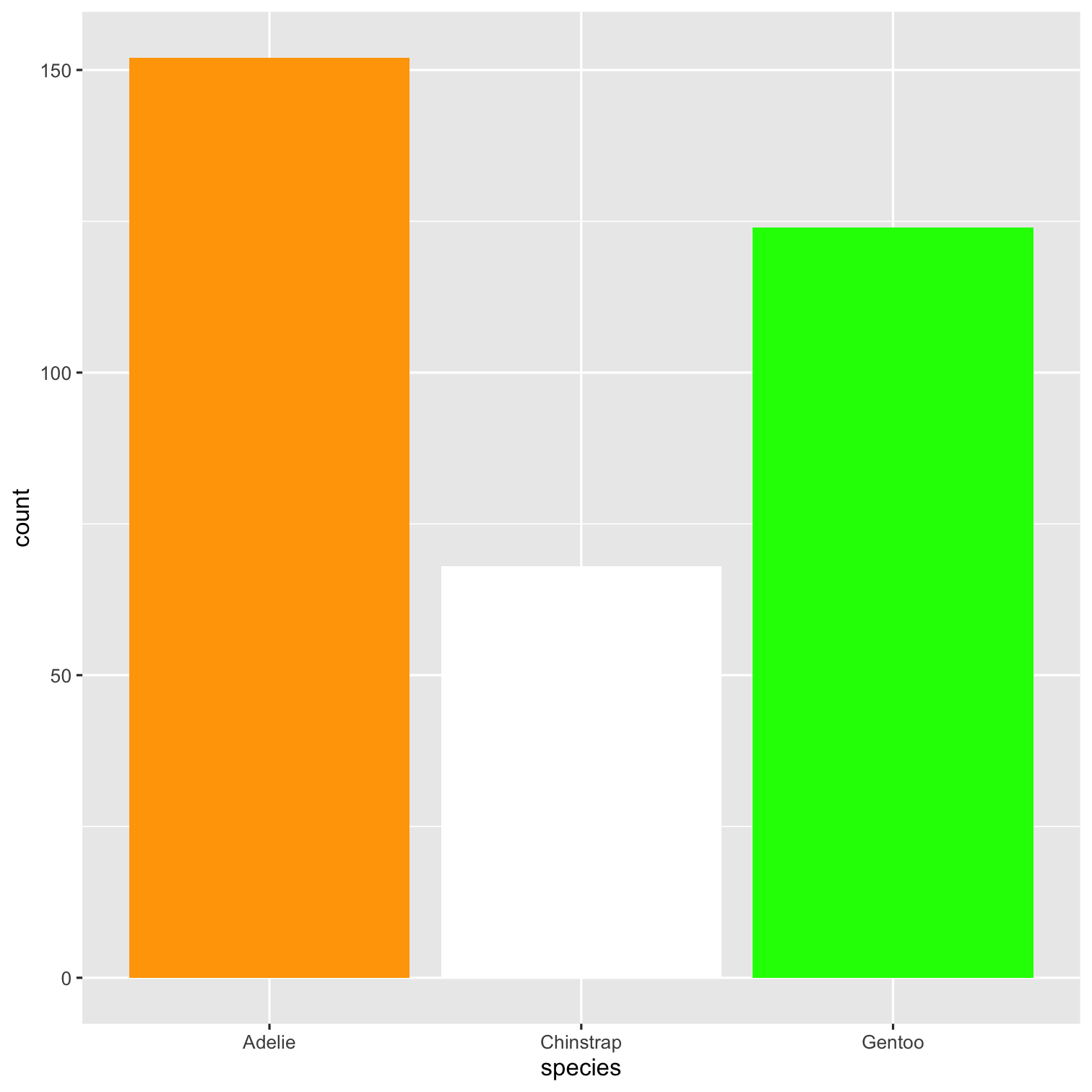
How to add color to bars?
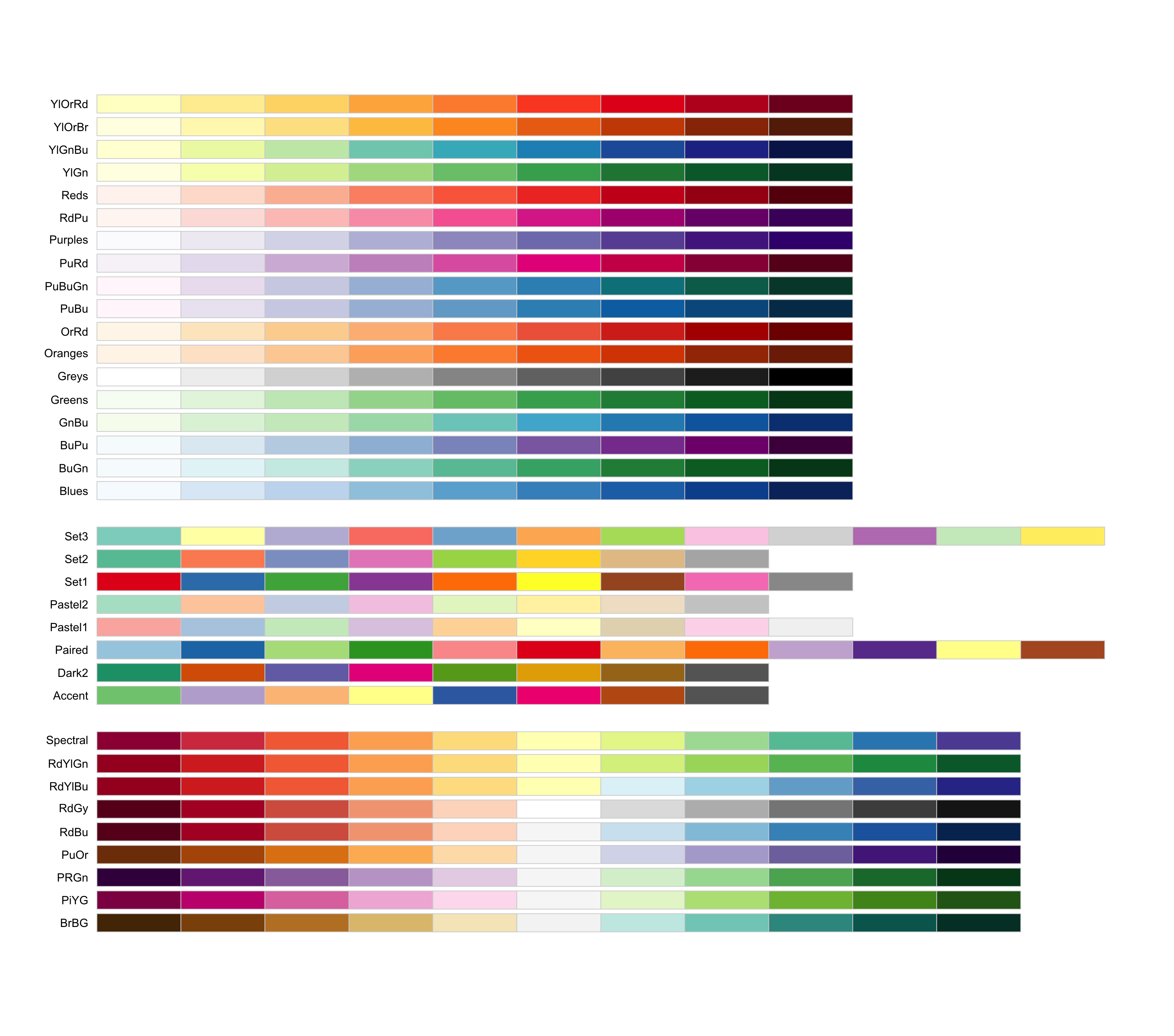
How to add color using palette? 🎨
🎨 Color Palette
- R package
RColorBrewer&wesanderson
How to remove legend or change its position?
How to plot title and axis titles?
How to control size of text?
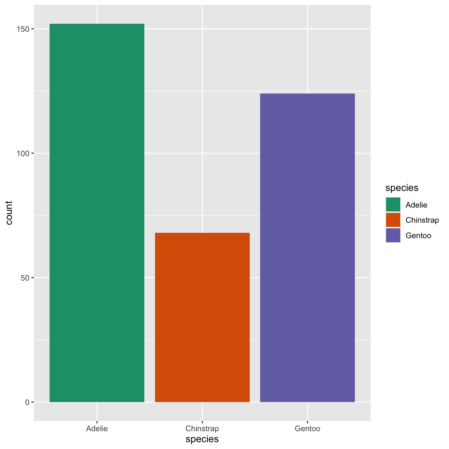
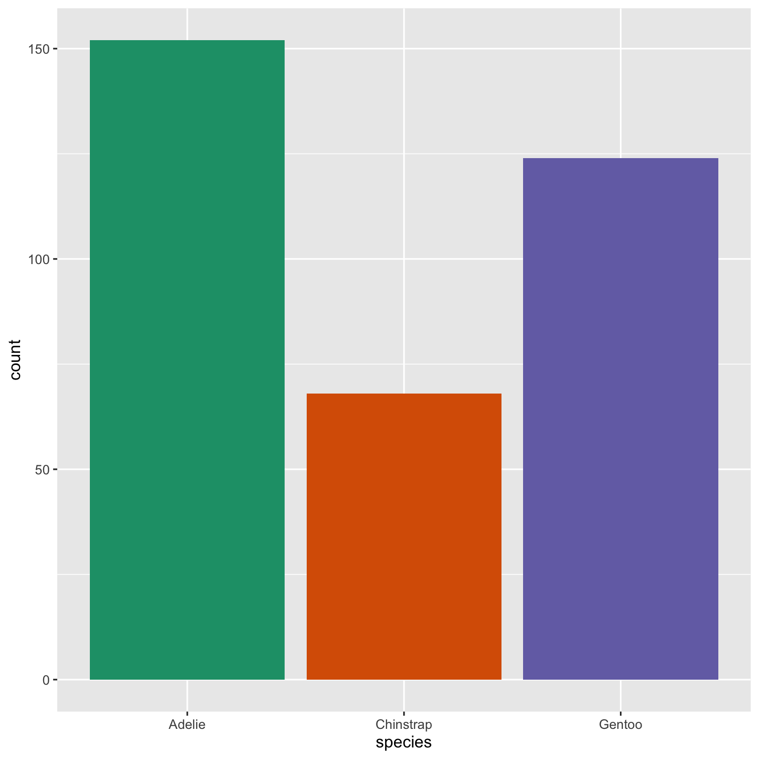
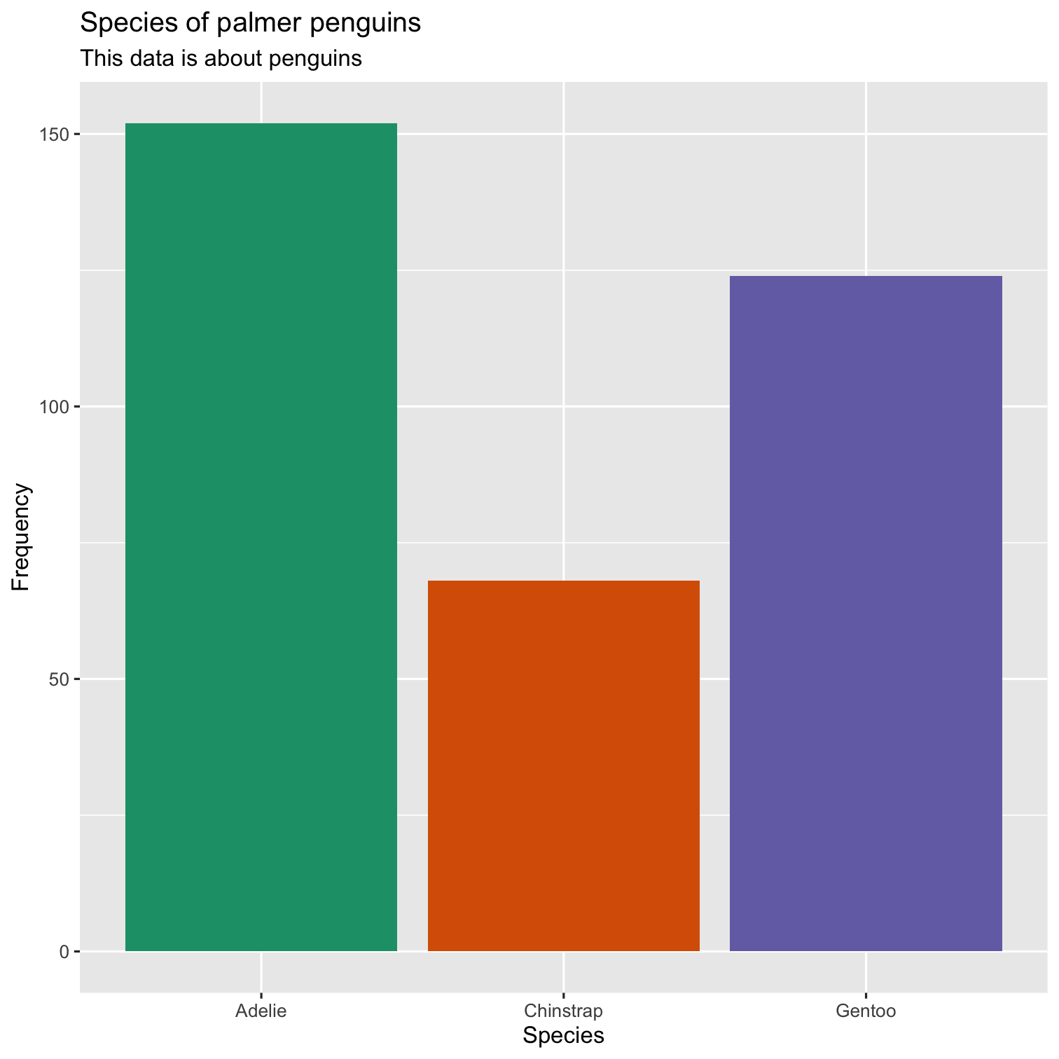
ggplot(data = penguins, mapping = aes(x = species, fill = species)) + geom_bar() + scale_fill_brewer(palette = "Dark2") + theme(legend.position = "none", text = element_text(size = 20)) + labs( title = "Species of palmer penguins", subtitle = "This data is about penguins", x = "Species", y = "Frequency" )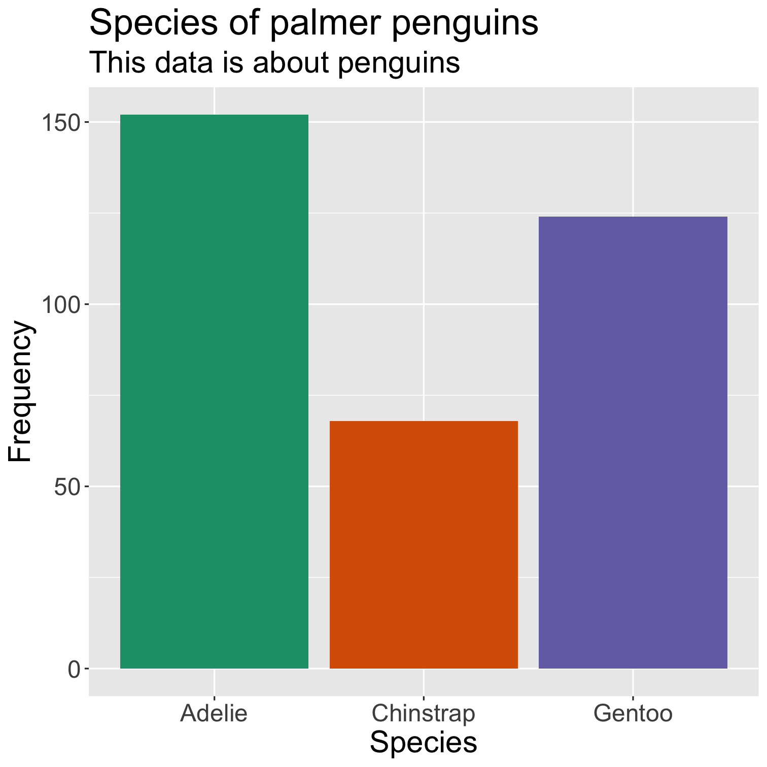
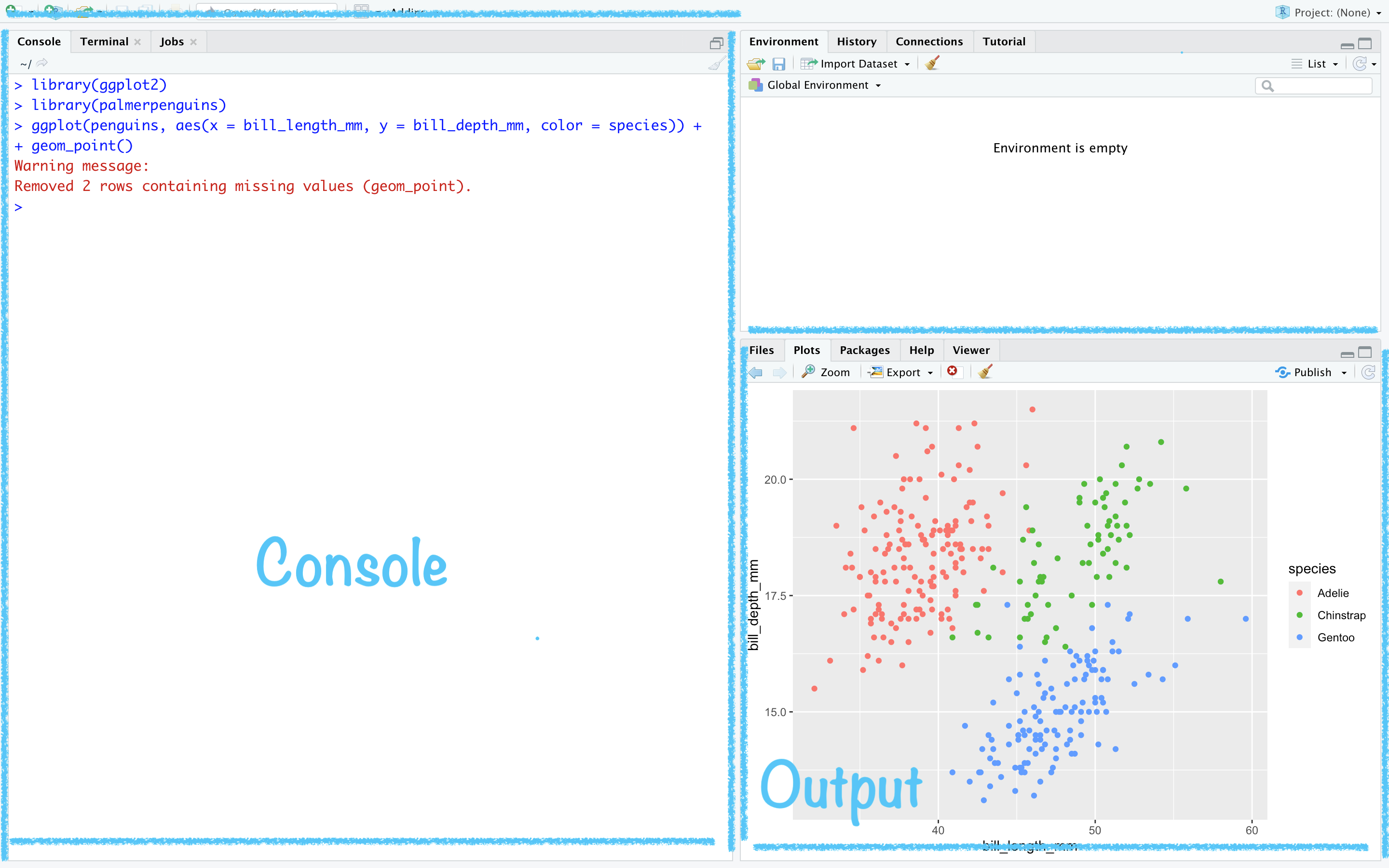
How to plot two numeric variables?
ggplot(data = penguins, mapping = aes(x = bill_length_mm, y = bill_depth_mm, color = species)) + geom_point() + scale_fill_brewer(palette = "Dark2") + theme(legend.position = "none", text = element_text(size = 20)) + labs( title = "Relationship between bill length \n& depth of palmer penguins", subtitle = "This data is about penguins", x = "Bill length (mm)", y = "Bith depth (mm)" )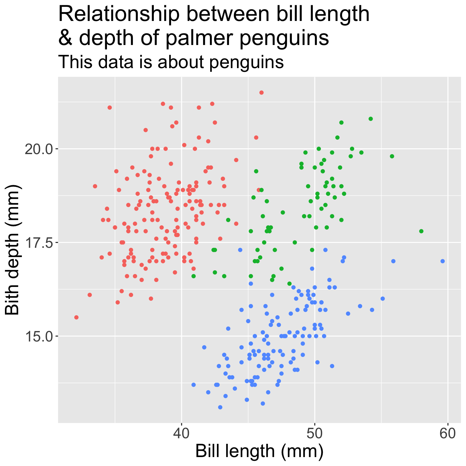
How to add themes to ggplot?
ggplot2 themes
https://ggplot2.tidyverse.org/reference/ggtheme.html
theme_gray()
theme_bw()
theme_linedraw()
theme_light()
theme_dark()
theme_minimal()
theme_classic()
theme_void()
theme_test()
ggplot(data = penguins, mapping = aes(x = bill_length_mm, y = bill_depth_mm, color = species)) + geom_point() + scale_fill_brewer(palette = "Dark2") + theme(legend.position = "none", text = element_text(size = 20)) + labs( title = "Relationship between bill length \n& depth of palmer penguins", subtitle = "This data is about penguins", x = "Bill length (mm)", y = "Bith depth (mm)" ) + theme_bw()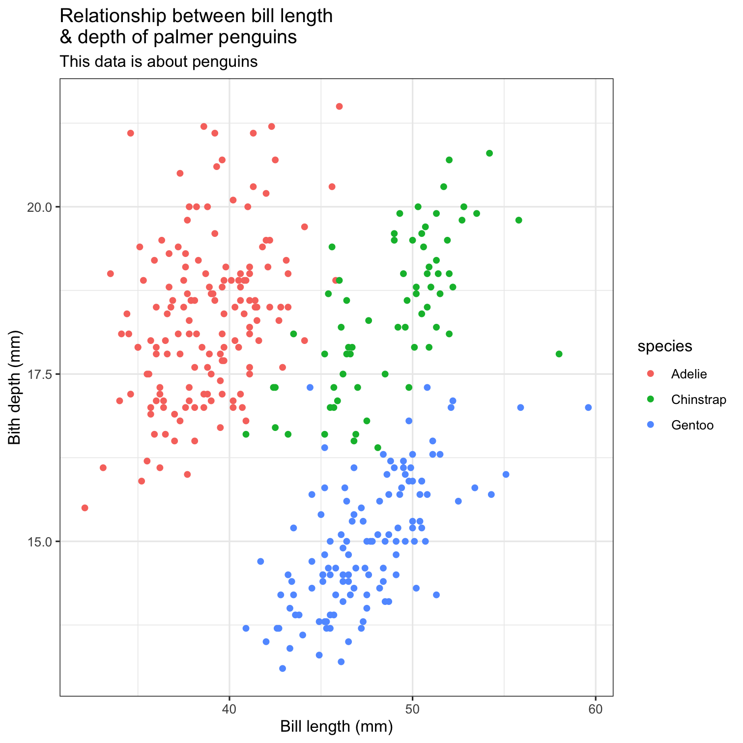
ggplot(data = penguins, mapping = aes(x = bill_length_mm, y = bill_depth_mm, color = species)) + geom_point() + scale_fill_brewer(palette = "Dark2") + theme(legend.position = "none", text = element_text(size = 20)) + labs( title = "Relationship between bill length \n& depth of palmer penguins", subtitle = "This data is about penguins", x = "Bill length (mm)", y = "Bith depth (mm)" ) + theme_classic()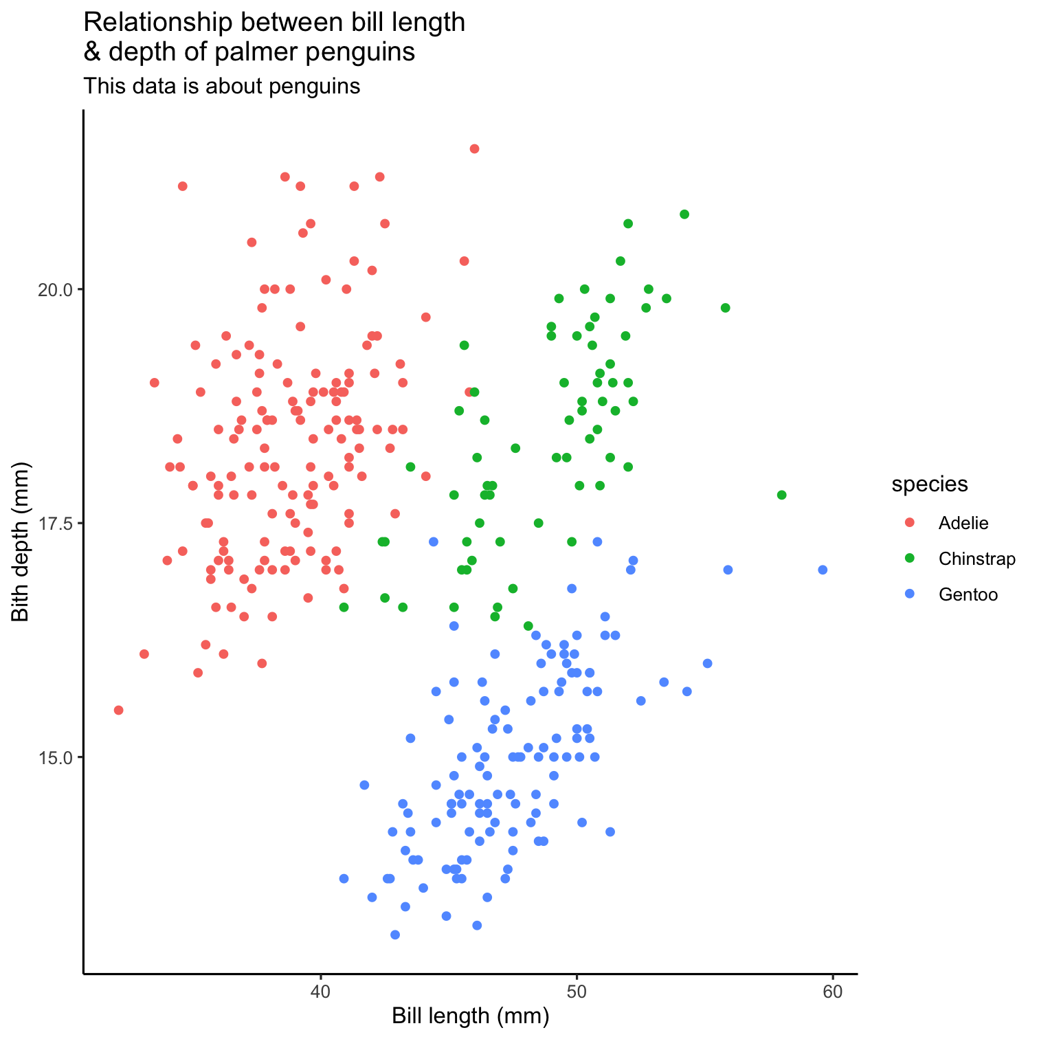
How to add regression line to ggplot?
ggplot(data = penguins, mapping = aes(x = flipper_length_mm, y = body_mass_g)) + geom_point() + theme(legend.position = "none", text = element_text(size = 24)) + labs( title = "Relationship between bill length \n& depth of palmer penguins", subtitle = "This data is about penguins", x = "Flipper length (mm)", y = "Body mass (gm)" ) + theme_classic() + geom_smooth()
More resources
ggplot2 book https://ggplot2-book.org/
CÉDRIC SCHERER https://www.cedricscherer.com/
ggplot2 cook book http://www.cookbook-r.com/
🙋🏽♀️🙋♂️
Q&A
Dynamic Wrangling
Using dplyr
Next Module - 4
Course Progress
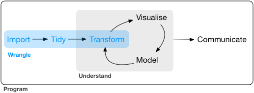
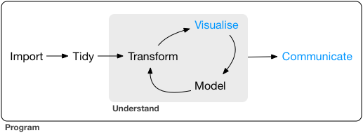
What is Data wrangling?
What is Data wrangling?
"data exploration and data manipulation" (Jesse Mostipak)
"tidying and transforming" (Hadley & Garrett)
What is Data wrangling?
"data exploration and data manipulation" (Jesse Mostipak)
"tidying and transforming" (Hadley & Garrett)
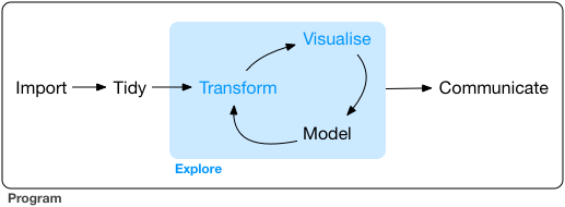
"Transforming" data means:
- "narrowing in on observations of interest ...
"Transforming" data means:
"narrowing in on observations of interest ...
creating new variables that are functions of existing variables ... and
"Transforming" data means:
"narrowing in on observations of interest ...
creating new variables that are functions of existing variables ... and
calculating a set of summary statistics."
R
Package
dplyr package
- "dplyr is a grammar of data manipulation"
dplyr package
"dplyr is a grammar of data manipulation"
"providing a consistent set of verbs that help you solve the most common data manipulation challenges:"
dplyr package
"dplyr is a grammar of data manipulation"
"providing a consistent set of verbs that help you solve the most common data manipulation challenges:"
Few important functions:
filter()select()mutate()arrange()summarise()
filter() function:
- Picks cases based on their values.
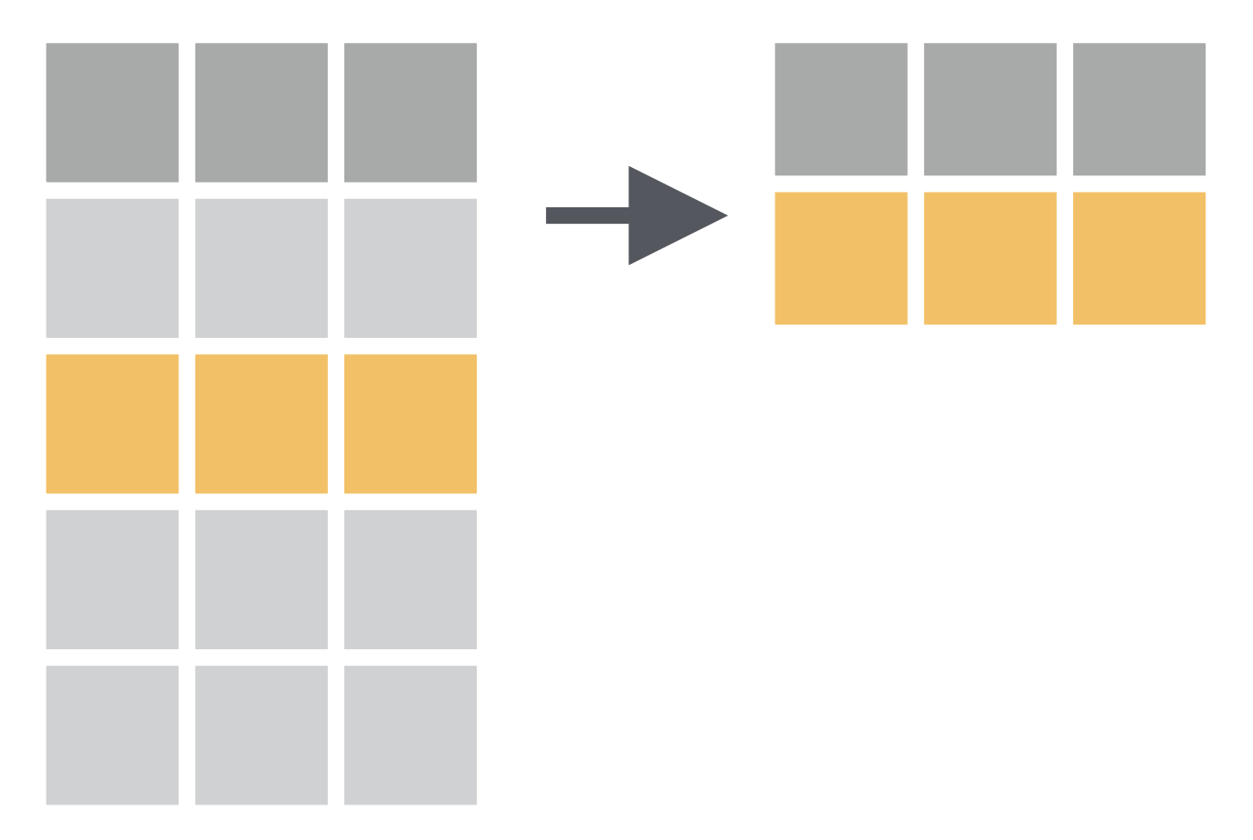
How to have a data of only Gentoo penguins?
# there are three species: Chinstrap, Gentoo, Adeliepenguins %>% filter(species == "Gentoo")## # A tibble: 124 × 8## species island bill_length_mm## <fct> <fct> <dbl>## 1 Gentoo Biscoe 46.1## 2 Gentoo Biscoe 50 ## 3 Gentoo Biscoe 48.7## 4 Gentoo Biscoe 50 ## 5 Gentoo Biscoe 47.6## 6 Gentoo Biscoe 46.5## 7 Gentoo Biscoe 45.4## 8 Gentoo Biscoe 46.7## 9 Gentoo Biscoe 43.3## 10 Gentoo Biscoe 46.8## # … with 114 more rows, and 5 more## # variables: bill_depth_mm <dbl>,## # flipper_length_mm <int>,## # body_mass_g <int>, sex <fct>,## # year <int># there are three species: Chinstrap, Gentoo, Adeliepraw <- read_csv("data/gentoo-penguins1.csv")praw %>% filter(species == "Gentoo") %>% summary() %>% kableExtra::kable()| species | island | bill_length_mm | bill_depth_mm | flipper_length_mm | body_mass_g | sex | year | |
|---|---|---|---|---|---|---|---|---|
| Length:124 | Length:124 | Min. :40.90 | Min. :13.10 | Min. :203.0 | Min. :3950 | Length:124 | Min. :2007 | |
| Class :character | Class :character | 1st Qu.:45.30 | 1st Qu.:14.20 | 1st Qu.:212.0 | 1st Qu.:4500 | Class :character | 1st Qu.:2007 | |
| Mode :character | Mode :character | Median :47.30 | Median :15.00 | Median :216.0 | Median :4925 | Mode :character | Median :2008 | |
| NA | NA | Mean :47.50 | Mean :14.98 | Mean :217.2 | Mean :4985 | NA | Mean :2008 | |
| NA | NA | 3rd Qu.:49.55 | 3rd Qu.:15.70 | 3rd Qu.:221.0 | 3rd Qu.:5400 | NA | 3rd Qu.:2009 | |
| NA | NA | Max. :59.60 | Max. :17.30 | Max. :231.0 | Max. :6050 | NA | Max. :2009 | |
| NA | NA | NA's :1 | NA's :1 | NA's :1 | NA's :1 | NA | NA |
How to export data file to your computer?
✋ WAIT! What is %>%
✋ WAIT! What is %>%
- this is called pipe (
%>%= control + shift + m)
✋ WAIT! What is %>%
this is called pipe (
%>%= control + shift + m)"a powerful tool for clearly expressing a sequence of multiple operations"
✋ WAIT! What is %>%
this is called pipe (
%>%= control + shift + m)"a powerful tool for clearly expressing a sequence of multiple operations"
interpret/read it as then.
penguins %>% filter(species == "Gentoo") %>% summary() %>% kableExtra::kable()Comparison: Relational Operators
x < y
Comparison: Relational Operators
x < y
x > y
Comparison: Relational Operators
x < y
x > y
x <= y
Comparison: Relational Operators
x < y
x > y
x <= y
x >= y
Comparison: Relational Operators
x < y
x > y
x <= y
x >= y
x == y (equal)
Comparison: Relational Operators
x < y
x > y
x <= y
x >= y
x == y (equal)
x != y (not equal)
How to have a data of penguins with bill length more than 43 mm?
penguins %>% filter(bill_length_mm > 43)## # A tibble: 188 × 8## species island bill_length_mm## <fct> <fct> <dbl>## 1 Adelie Torgersen 46 ## 2 Adelie Dream 44.1## 3 Adelie Torgersen 45.8## 4 Adelie Dream 43.2## 5 Adelie Biscoe 43.2## 6 Adelie Biscoe 45.6## 7 Adelie Torgersen 44.1## 8 Adelie Torgersen 43.1## 9 Gentoo Biscoe 46.1## 10 Gentoo Biscoe 50 ## # … with 178 more rows, and 5 more## # variables: bill_depth_mm <dbl>,## # flipper_length_mm <int>,## # body_mass_g <int>, sex <fct>,## # year <int>How to have a data of Gentoo penguins with bill length more than 50 mm?
penguins %>% filter(species == "Gentoo", bill_length_mm > 55)## # A tibble: 3 × 8## species island bill_length_mm## <fct> <fct> <dbl>## 1 Gentoo Biscoe 59.6## 2 Gentoo Biscoe 55.9## 3 Gentoo Biscoe 55.1## # … with 5 more variables:## # bill_depth_mm <dbl>,## # flipper_length_mm <int>,## # body_mass_g <int>, sex <fct>,## # year <int>How to have data of non-Gentoo penguins with bill length more than 45 mm and weight more than 4 kg?
penguins %>% filter(species != "Gentoo", bill_length_mm > 45, body_mass_g > 4000)## # A tibble: 18 × 8## species island bill_length_mm## <fct> <fct> <dbl>## 1 Adelie Torgersen 46 ## 2 Adelie Torgersen 45.8## 3 Adelie Biscoe 45.6## 4 Chinstrap Dream 46 ## 5 Chinstrap Dream 52 ## 6 Chinstrap Dream 50.5## 7 Chinstrap Dream 49.2## 8 Chinstrap Dream 52 ## 9 Chinstrap Dream 52.8## 10 Chinstrap Dream 54.2## 11 Chinstrap Dream 51 ## 12 Chinstrap Dream 52 ## 13 Chinstrap Dream 53.5## 14 Chinstrap Dream 50.8## 15 Chinstrap Dream 49 ## 16 Chinstrap Dream 50.7## 17 Chinstrap Dream 49.3## 18 Chinstrap Dream 50.8## # … with 5 more variables:## # bill_depth_mm <dbl>,## # flipper_length_mm <int>,## # body_mass_g <int>, sex <fct>,## # year <int>How to have only top or bottom rows from data?
penguins %>% filter(species != "Gentoo", bill_length_mm > 45, body_mass_g > 4000) %>% head()## # A tibble: 6 × 8## species island bill_length_mm## <fct> <fct> <dbl>## 1 Adelie Torgersen 46 ## 2 Adelie Torgersen 45.8## 3 Adelie Biscoe 45.6## 4 Chinstrap Dream 46 ## 5 Chinstrap Dream 52 ## 6 Chinstrap Dream 50.5## # … with 5 more variables:## # bill_depth_mm <dbl>,## # flipper_length_mm <int>,## # body_mass_g <int>, sex <fct>,## # year <int>penguins %>% filter(species != "Gentoo", bill_length_mm > 45, body_mass_g > 4000) %>% tail(3)## # A tibble: 3 × 8## species island bill_length_mm## <fct> <fct> <dbl>## 1 Chinstrap Dream 50.7## 2 Chinstrap Dream 49.3## 3 Chinstrap Dream 50.8## # … with 5 more variables:## # bill_depth_mm <dbl>,## # flipper_length_mm <int>,## # body_mass_g <int>, sex <fct>,## # year <int>🧠 YOUR TURN
10:00
How many Chinstrap penguins are with bill length more than 45 mm and weight more than 4 kg?
penguins %>% filter(species == "Chinstrap", bill_length_mm > 45, body_mass_g > 4000) %>% head()## # A tibble: 6 × 8## species island bill_length_mm## <fct> <fct> <dbl>## 1 Chinstrap Dream 46 ## 2 Chinstrap Dream 52 ## 3 Chinstrap Dream 50.5## 4 Chinstrap Dream 49.2## 5 Chinstrap Dream 52 ## 6 Chinstrap Dream 52.8## # … with 5 more variables:## # bill_depth_mm <dbl>,## # flipper_length_mm <int>,## # body_mass_g <int>, sex <fct>,## # year <int>select() function: Chooses rows based on column values.
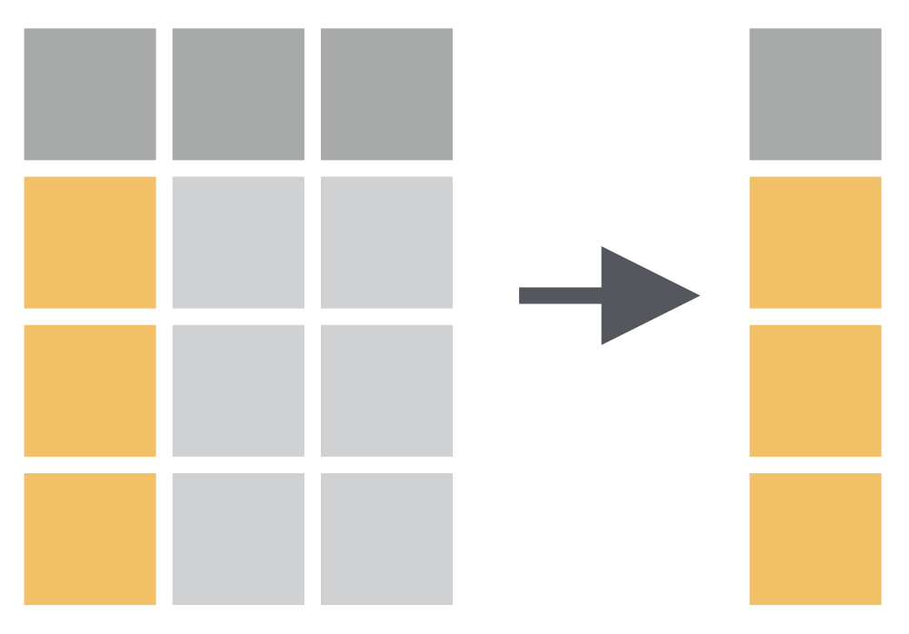
How to have only species variable in data?
How to have a specific range of variables in data?
penguins %>% select(species : bill_depth_mm)## # A tibble: 344 × 4## species island bill_length_mm## <fct> <fct> <dbl>## 1 Adelie Torgersen 39.1## 2 Adelie Torgersen 39.5## 3 Adelie Torgersen 40.3## 4 Adelie Torgersen NA ## 5 Adelie Torgersen 36.7## 6 Adelie Torgersen 39.3## 7 Adelie Torgersen 38.9## 8 Adelie Torgersen 39.2## 9 Adelie Torgersen 34.1## 10 Adelie Torgersen 42 ## # … with 334 more rows, and 1 more## # variable: bill_depth_mm <dbl>How to have variables based upon their location in data?
penguins %>% select(4:8)## # A tibble: 344 × 5## bill_depth_mm flipper_length_mm## <dbl> <int>## 1 18.7 181## 2 17.4 186## 3 18 195## 4 NA NA## 5 19.3 193## 6 20.6 190## 7 17.8 181## 8 19.6 195## 9 18.1 193## 10 20.2 190## # … with 334 more rows, and 3 more## # variables: body_mass_g <int>,## # sex <fct>, year <int>How to have specific variables in data?
penguins %>% select(species, body_mass_g, year)## # A tibble: 344 × 3## species body_mass_g year## <fct> <int> <int>## 1 Adelie 3750 2007## 2 Adelie 3800 2007## 3 Adelie 3250 2007## 4 Adelie NA 2007## 5 Adelie 3450 2007## 6 Adelie 3650 2007## 7 Adelie 3625 2007## 8 Adelie 4675 2007## 9 Adelie 3475 2007## 10 Adelie 4250 2007## # … with 334 more rowspenguins %>% select(-c(species, body_mass_g, year))## # A tibble: 344 × 5## island bill_length_mm bill_depth_mm## <fct> <dbl> <dbl>## 1 Torgersen 39.1 18.7## 2 Torgersen 39.5 17.4## 3 Torgersen 40.3 18 ## 4 Torgersen NA NA ## 5 Torgersen 36.7 19.3## 6 Torgersen 39.3 20.6## 7 Torgersen 38.9 17.8## 8 Torgersen 39.2 19.6## 9 Torgersen 34.1 18.1## 10 Torgersen 42 20.2## # … with 334 more rows, and 2 more## # variables: flipper_length_mm <int>,## # sex <fct>mutate() function: Adds new variables that are functions of existing variables
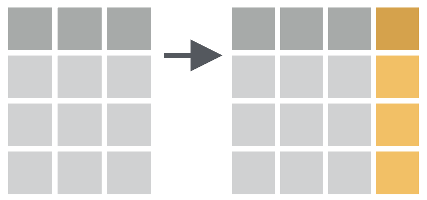
How to convert penguin body mass from grams to kilograms?
penguins %>% mutate(body_mass_kg = body_mass_g / 1000)## # A tibble: 344 × 9## species island bill_length_mm## <fct> <fct> <dbl>## 1 Adelie Torgersen 39.1## 2 Adelie Torgersen 39.5## 3 Adelie Torgersen 40.3## 4 Adelie Torgersen NA ## 5 Adelie Torgersen 36.7## 6 Adelie Torgersen 39.3## 7 Adelie Torgersen 38.9## 8 Adelie Torgersen 39.2## 9 Adelie Torgersen 34.1## 10 Adelie Torgersen 42 ## # … with 334 more rows, and 6 more## # variables: bill_depth_mm <dbl>,## # flipper_length_mm <int>,## # body_mass_g <int>, sex <fct>,## # year <int>, body_mass_kg <dbl>penguins %>% select(body_mass_g) %>% mutate(body_mass_kg = body_mass_g / 1000)## # A tibble: 344 × 2## body_mass_g body_mass_kg## <int> <dbl>## 1 3750 3.75## 2 3800 3.8 ## 3 3250 3.25## 4 NA NA ## 5 3450 3.45## 6 3650 3.65## 7 3625 3.62## 8 4675 4.68## 9 3475 3.48## 10 4250 4.25## # … with 334 more rowspenguins %>% mutate(body_mass_kg = body_mass_g / 1000, bill = bill_length_mm * bill_depth_mm)## # A tibble: 344 × 10## species island bill_length_mm## <fct> <fct> <dbl>## 1 Adelie Torgersen 39.1## 2 Adelie Torgersen 39.5## 3 Adelie Torgersen 40.3## 4 Adelie Torgersen NA ## 5 Adelie Torgersen 36.7## 6 Adelie Torgersen 39.3## 7 Adelie Torgersen 38.9## 8 Adelie Torgersen 39.2## 9 Adelie Torgersen 34.1## 10 Adelie Torgersen 42 ## # … with 334 more rows, and 7 more## # variables: bill_depth_mm <dbl>,## # flipper_length_mm <int>,## # body_mass_g <int>, sex <fct>,## # year <int>, body_mass_kg <dbl>,## # bill <dbl>penguins %>% mutate(body_mass_kg = body_mass_g / 1000, bill = bill_length_mm * bill_depth_mm) %>% select(body_mass_kg, bill)## # A tibble: 344 × 2## body_mass_kg bill## <dbl> <dbl>## 1 3.75 731.## 2 3.8 687.## 3 3.25 725.## 4 NA NA ## 5 3.45 708.## 6 3.65 810.## 7 3.62 692.## 8 4.68 768.## 9 3.48 617.## 10 4.25 848.## # … with 334 more rowsarrange() function: Changes the order of the rows.
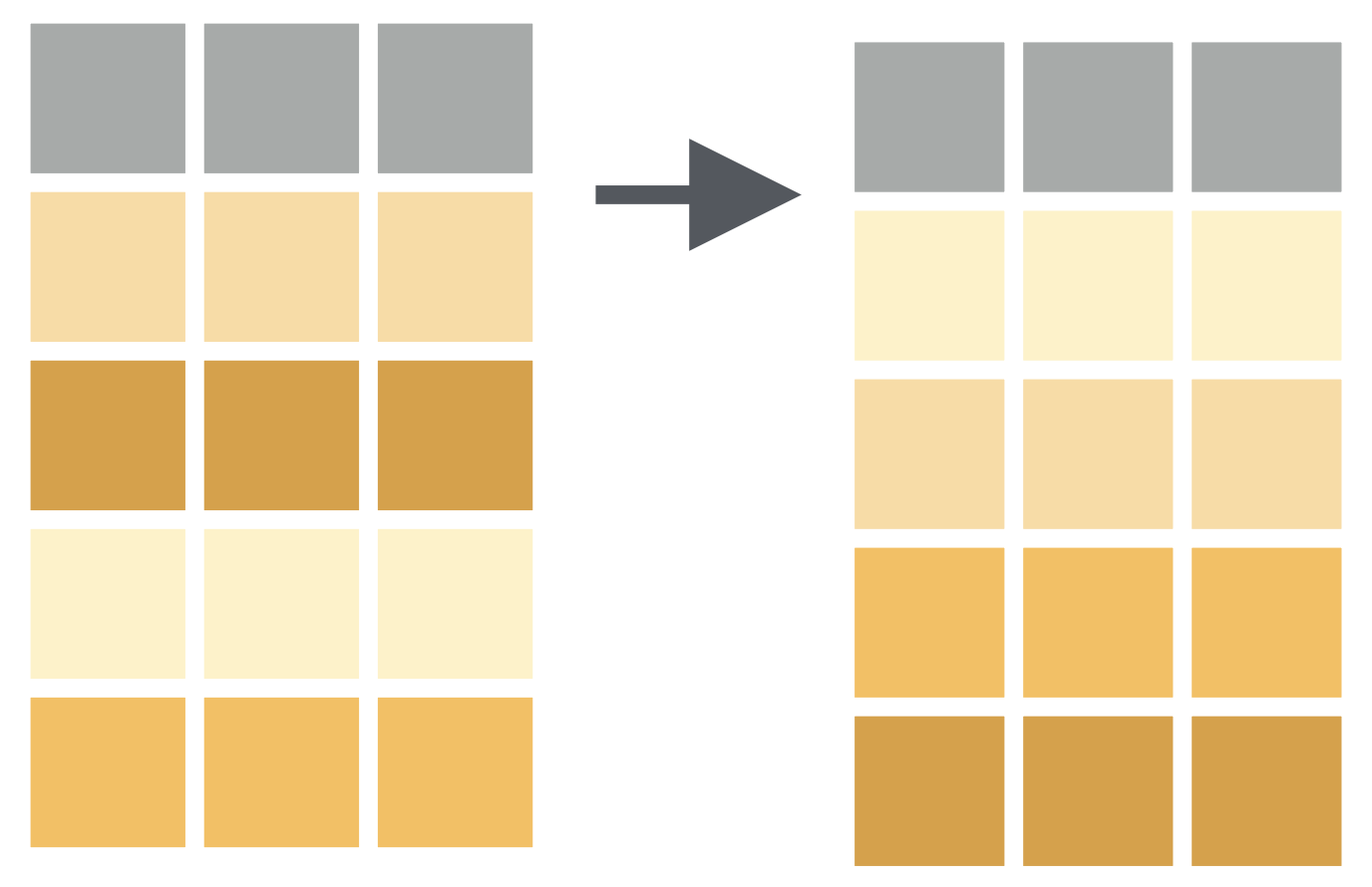
How to have data arranged by the ascending order of bill length of penguins?
penguins %>% arrange(bill_length_mm)## # A tibble: 344 × 8## species island bill_length_mm## <fct> <fct> <dbl>## 1 Adelie Dream 32.1## 2 Adelie Dream 33.1## 3 Adelie Torgersen 33.5## 4 Adelie Dream 34 ## 5 Adelie Torgersen 34.1## 6 Adelie Torgersen 34.4## 7 Adelie Biscoe 34.5## 8 Adelie Torgersen 34.6## 9 Adelie Torgersen 34.6## 10 Adelie Biscoe 35 ## # … with 334 more rows, and 5 more## # variables: bill_depth_mm <dbl>,## # flipper_length_mm <int>,## # body_mass_g <int>, sex <fct>,## # year <int>penguins %>% arrange(desc(bill_length_mm))## # A tibble: 344 × 8## species island bill_length_mm## <fct> <fct> <dbl>## 1 Gentoo Biscoe 59.6## 2 Chinstrap Dream 58 ## 3 Gentoo Biscoe 55.9## 4 Chinstrap Dream 55.8## 5 Gentoo Biscoe 55.1## 6 Gentoo Biscoe 54.3## 7 Chinstrap Dream 54.2## 8 Chinstrap Dream 53.5## 9 Gentoo Biscoe 53.4## 10 Chinstrap Dream 52.8## # … with 334 more rows, and 5 more## # variables: bill_depth_mm <dbl>,## # flipper_length_mm <int>,## # body_mass_g <int>, sex <fct>,## # year <int>penguins %>% arrange(species)## # A tibble: 344 × 8## species island bill_length_mm## <fct> <fct> <dbl>## 1 Adelie Torgersen 39.1## 2 Adelie Torgersen 39.5## 3 Adelie Torgersen 40.3## 4 Adelie Torgersen NA ## 5 Adelie Torgersen 36.7## 6 Adelie Torgersen 39.3## 7 Adelie Torgersen 38.9## 8 Adelie Torgersen 39.2## 9 Adelie Torgersen 34.1## 10 Adelie Torgersen 42 ## # … with 334 more rows, and 5 more## # variables: bill_depth_mm <dbl>,## # flipper_length_mm <int>,## # body_mass_g <int>, sex <fct>,## # year <int>summarise() function
summarise() function: Chooses rows based on column values.
How to find mean bill length of all penguins?
How to find species-wise mean bill length of penguins?
How to find species-wise mean bill length of penguins and total number of penguins in each species?
🙋🏽♀️🙋♂️
Q&A
Slide Crafting
using xaringan
Next Module - 5
R
Package
xaringan
- xaringan package to be a Presentation Ninja 🤺
xaringan
xaringan package to be a Presentation Ninja 🤺
"for creating slideshows with remark.js through R Markdown"
Packages required:
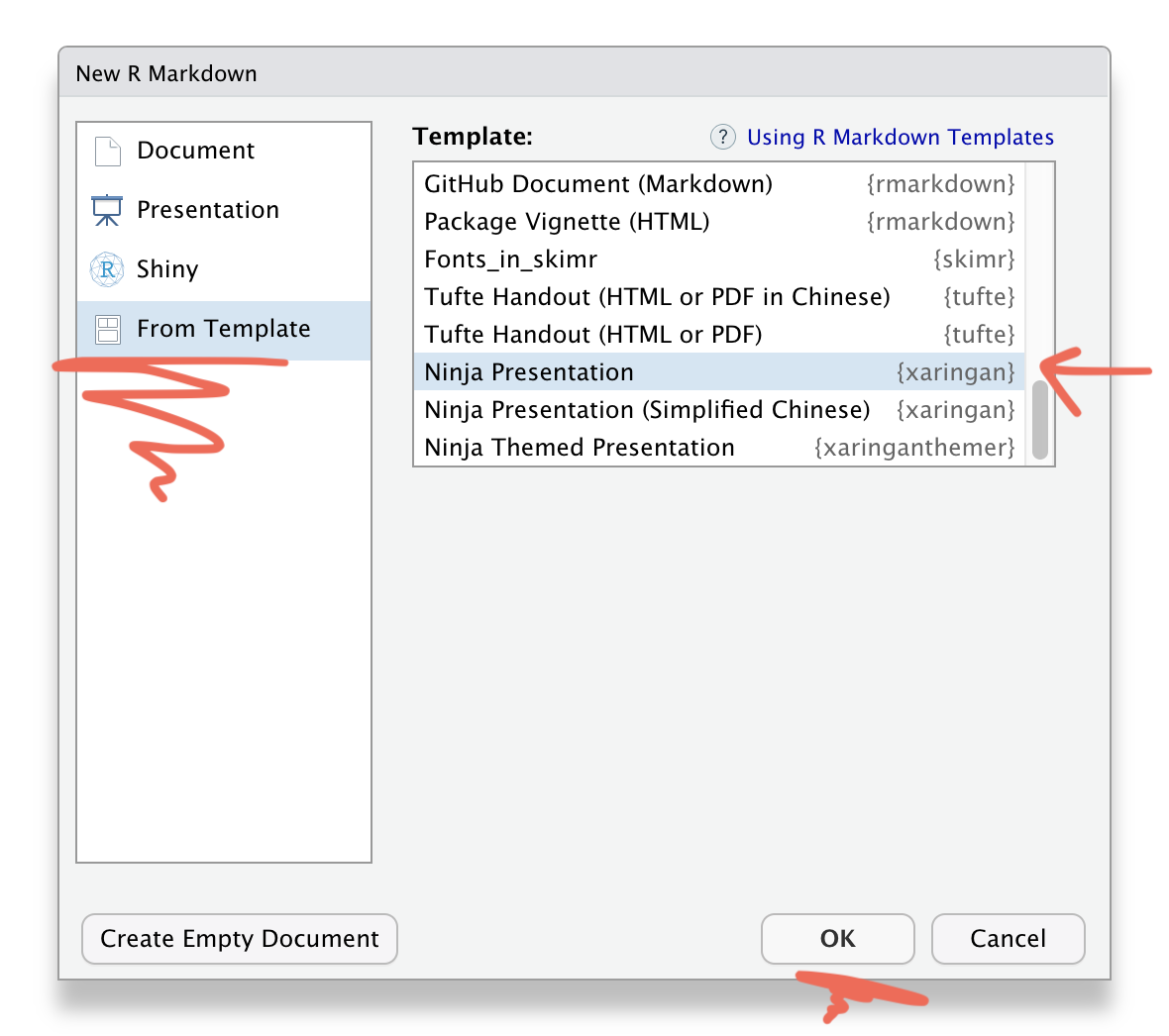
library(palmerpenguins) # to access penguin datalibrary(xaringan)library(xaringanthemer)library(xaringanExtra)File ⟶ New File ⟶ R Markdown

Template → Ninja Presentation
Save this Rmd file
Addins → Inifinite Moon Reader
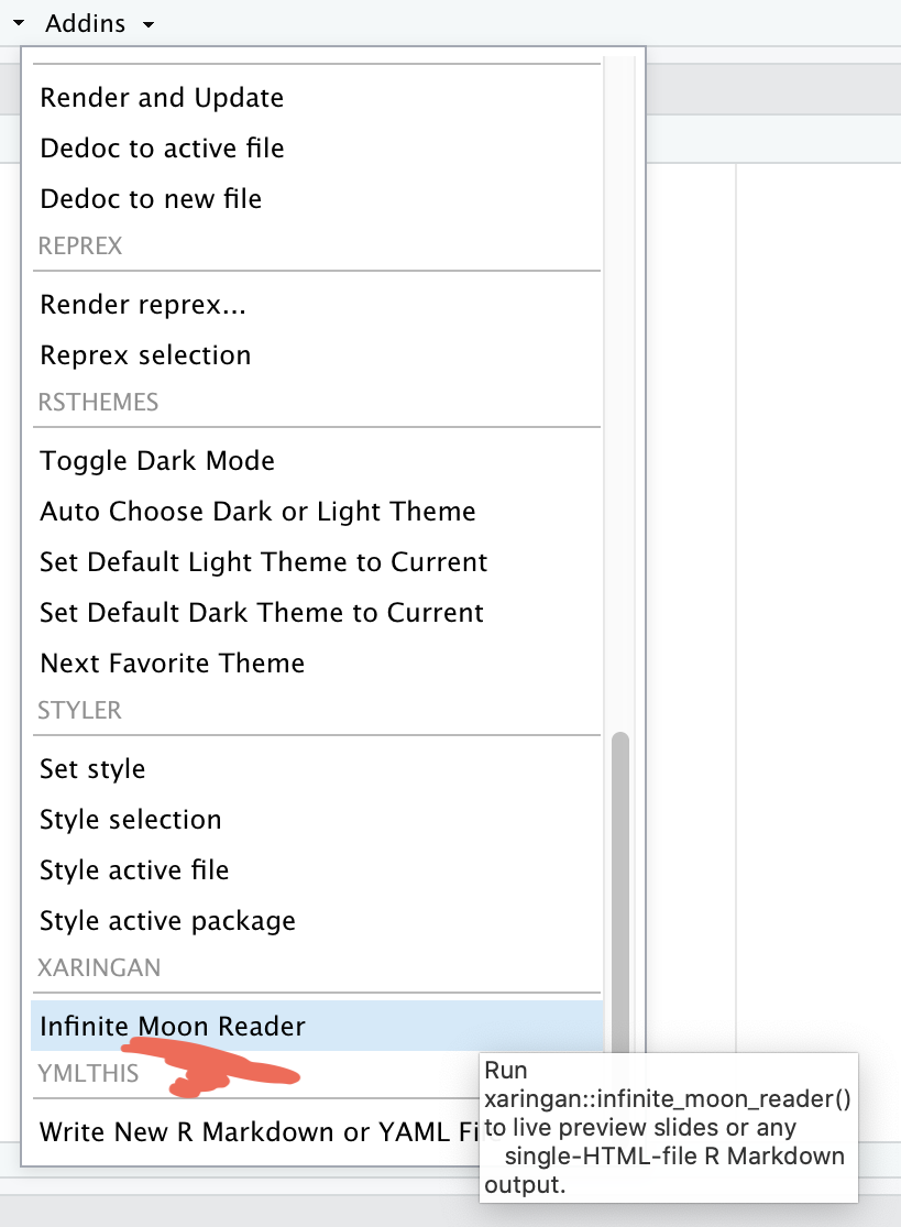
Addins → Inifinite Moon Reader
xaringan output
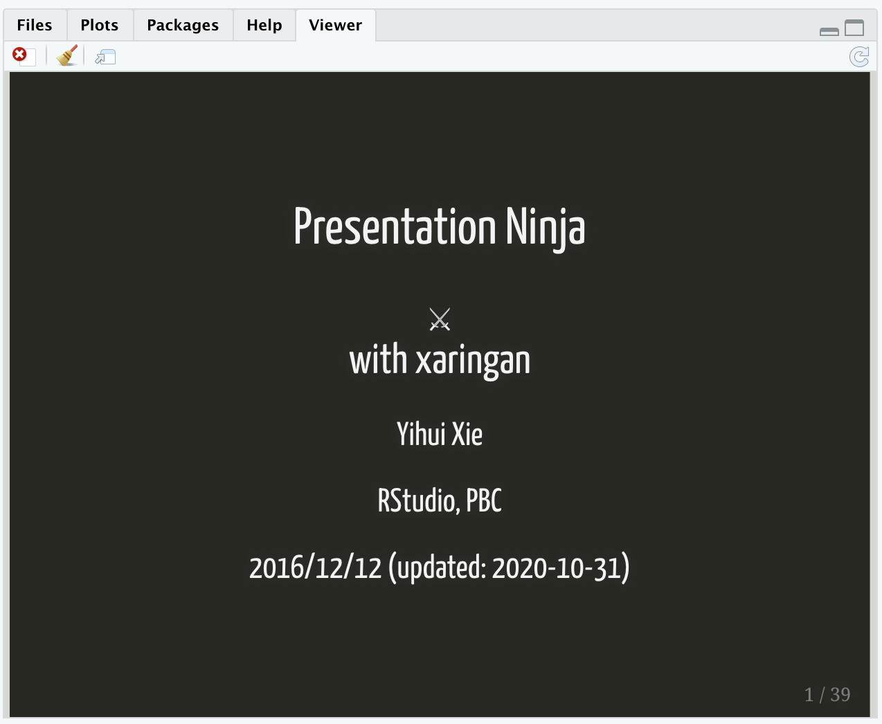
Addins → Inifinite Moon Reader
xaringan slide → browser
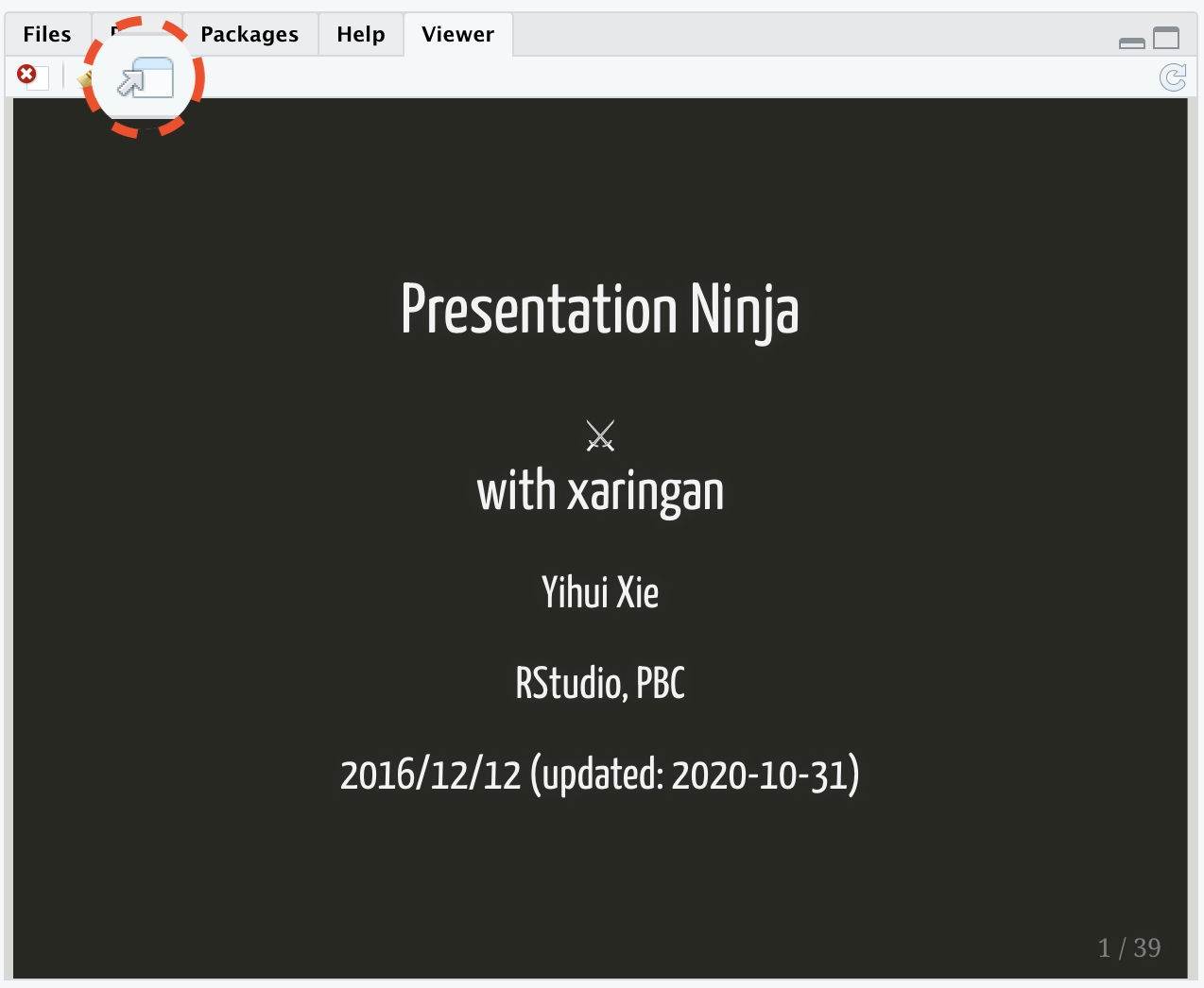
Addins → Inifinite Moon Reader
xaringan slide → browser
- We need to click
Inifinite Moon Readeronly to start the slideshow. To see the changes made in the slides just save the documentctrl + s
Using xaringan how to:
Using xaringan how to:
- create a new slide
Using xaringan how to:
create a new slide
hide an existing slide
Using xaringan how to:
create a new slide
hide an existing slide
heading, subheadings, points and normal text
Using xaringan how to:
create a new slide
hide an existing slide
heading, subheadings, points and normal text
include images
Using xaringan how to:
create a new slide
hide an existing slide
heading, subheadings, points and normal text
include images
- as background
Using xaringan how to:
create a new slide
hide an existing slide
heading, subheadings, points and normal text
include images
- as background
- as part of slide
Using xaringan how to:
create a new slide
hide an existing slide
heading, subheadings, points and normal text
include images
- as background
- as part of slide
make plots
Using xaringan how to:
create a new slide
hide an existing slide
heading, subheadings, points and normal text
include images
- as background
- as part of slide
make plots
include tables
Using xaringan how to:
create a new slide
hide an existing slide
heading, subheadings, points and normal text
include images
- as background
- as part of slide
make plots
include tables
in-text R output
Using xaringan how to:
create a new slide
hide an existing slide
heading, subheadings, points and normal text
include images
- as background
- as part of slide
make plots
include tables
in-text R output
create columns
- Use
---to create a new slide
Use
---to create a new slideexclude:trueTo hide an existing slide
Use
---to create a new slideexclude:trueTo hide an existing slideSlide text sizes:
Use
---to create a new slideexclude:trueTo hide an existing slideSlide text sizes:
#for main heading
Use
---to create a new slideexclude:trueTo hide an existing slideSlide text sizes:
#for main heading##for sub-heading
Use
---to create a new slideexclude:trueTo hide an existing slideSlide text sizes:
#for main heading##for sub-heading####for sub-sub-heading
Use
---to create a new slideexclude:trueTo hide an existing slideSlide text sizes:
#for main heading##for sub-heading####for sub-sub-heading
- indented
*for sub-point1 - indented
*for sub-point2 - indented
*for sub-point3
Use
---to create a new slideexclude:trueTo hide an existing slideSlide text sizes:
#for main heading##for sub-heading####for sub-sub-heading
- indented
*for sub-point1 - indented
*for sub-point2 - indented
*for sub-point3
-for normal text size
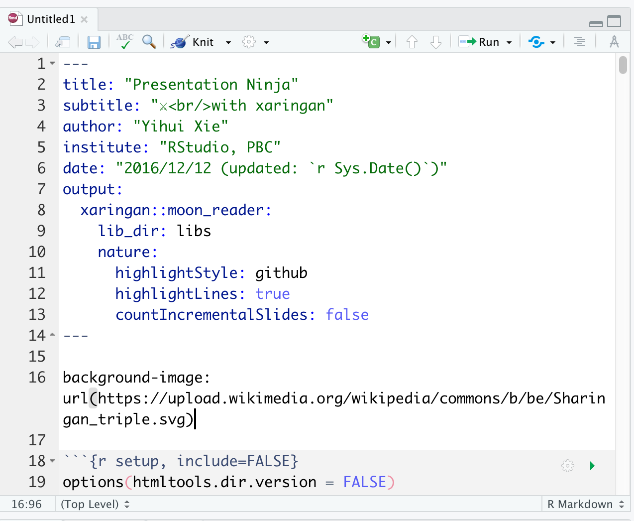
To include images using:
CSS background option:
To include images using:
CSS background option:
background-image: url("path of the image")= path of the image
To include images using:
CSS background option:
background-image: url("path of the image")= path of the imagebackground-size: contain, cover, 50%, 70%= size of the image
To include images using:
CSS background option:
background-image: url("path of the image")= path of the imagebackground-size: contain, cover, 50%, 70%= size of the imagebackground-position: left top= position of the image
To include images using:
knitr chunk option:
knitr::include_graphics("path of the image")To include plots
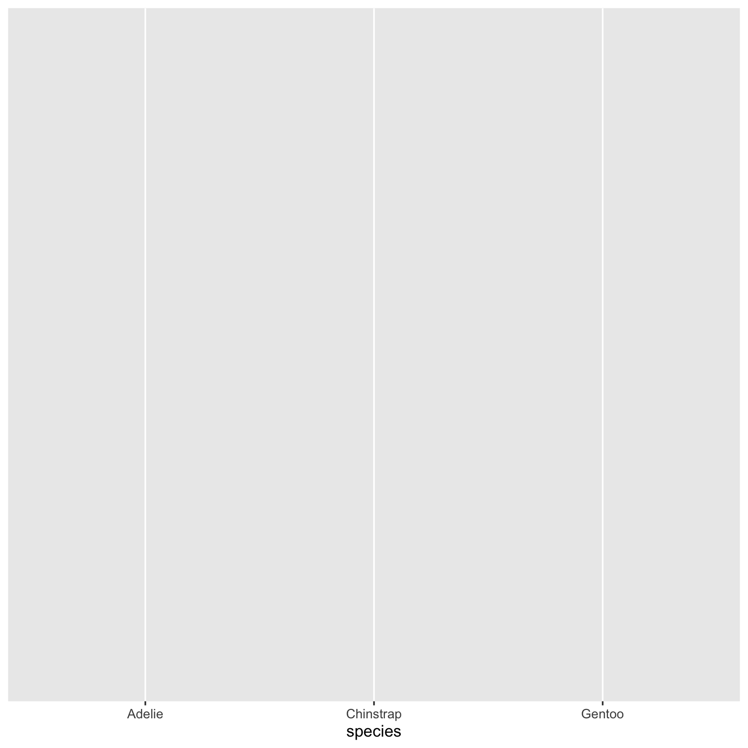
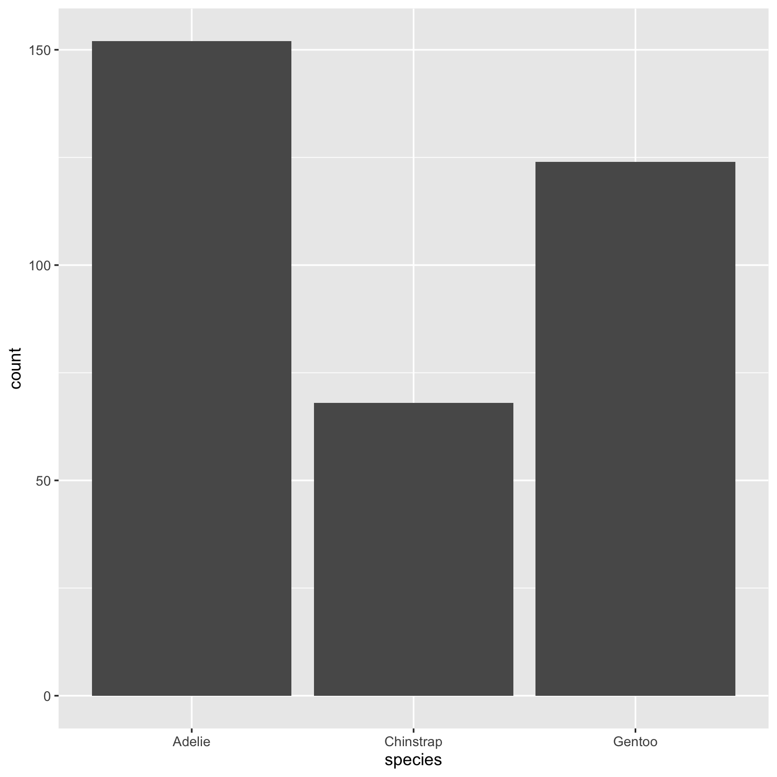
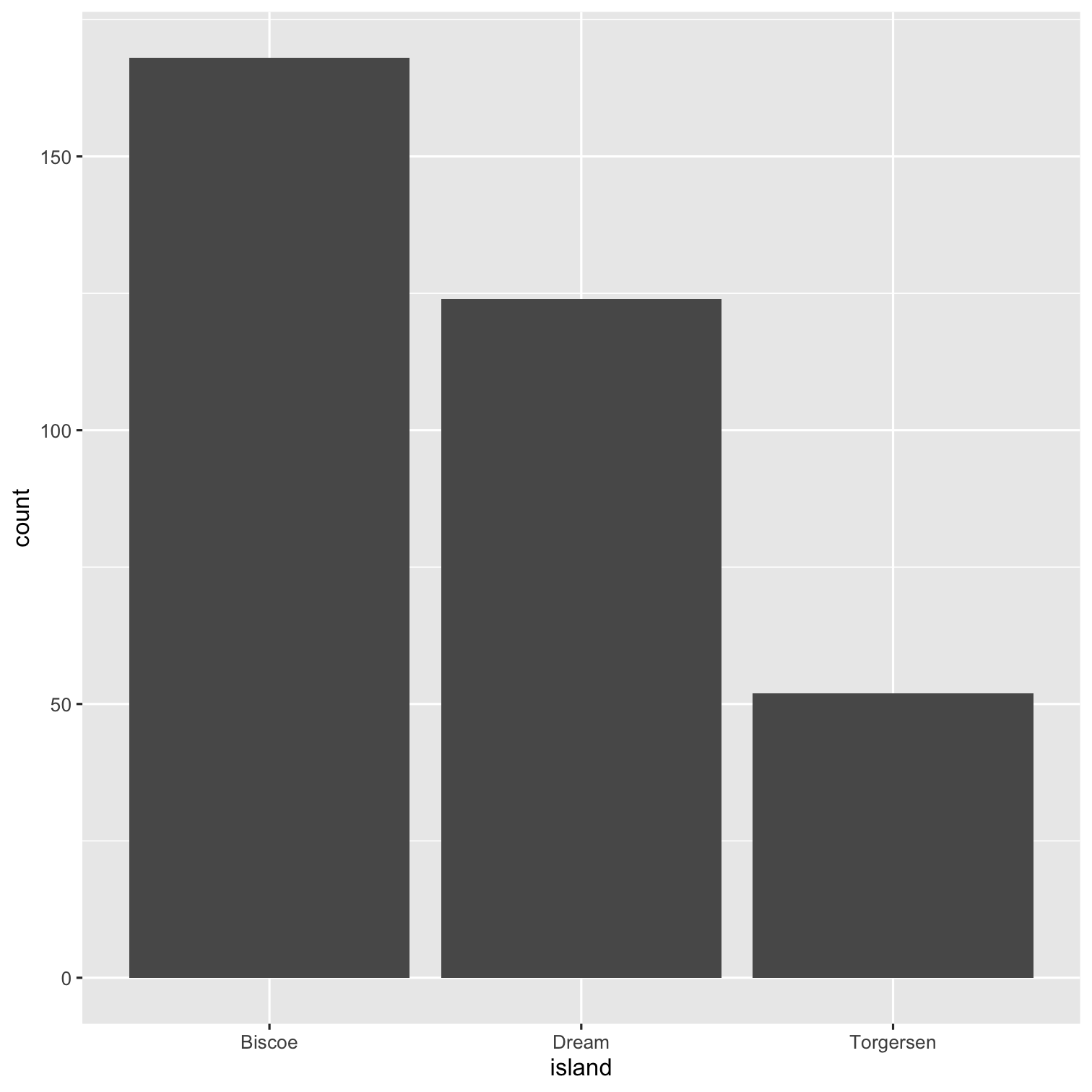
library(palmerpenguins)ggplot(penguins, aes(x = species)) + geom_bar()To include tables
library(kableExtra)library(tidyverse)penguins %>% drop_na() %>% head() %>% kable()| species | island | bill_length_mm | bill_depth_mm | flipper_length_mm | body_mass_g | sex | year |
|---|---|---|---|---|---|---|---|
| Adelie | Torgersen | 39.1 | 18.7 | 181 | 3750 | male | 2007 |
| Adelie | Torgersen | 39.5 | 17.4 | 186 | 3800 | female | 2007 |
| Adelie | Torgersen | 40.3 | 18.0 | 195 | 3250 | female | 2007 |
| Adelie | Torgersen | 36.7 | 19.3 | 193 | 3450 | female | 2007 |
| Adelie | Torgersen | 39.3 | 20.6 | 190 | 3650 | male | 2007 |
| Adelie | Torgersen | 38.9 | 17.8 | 181 | 3625 | female | 2007 |
In-text R output
- penguins data have a sample of n = 344 on total 8 variables.
In-text R output
penguins data have a sample of n = 344 on total 8 variables.
math expressions
a+b=σ−∑x22
Column division of slide
- left column
a
- b
- c
- right column
- apple
- boy
- cat
Slide class
- class can be assigned to each slide
Slide class
class can be assigned to each slide
it decides how all elements of one particular slide will look like
Slide class
class can be assigned to each slide
it decides how all elements of one particular slide will look like
class: center
Slide class
class can be assigned to each slide
it decides how all elements of one particular slide will look like
class: center, middle, inverse, right
Extend the power of xaringan:
Extend the power of xaringan:
using R packages like xaringanExtra
learn little about CSS
use cheatsheets